HyperLogLog++: Google’s Take On Engineering HLL

Matt Abrams recently pointed me to Google’s excellent paper “HyperLogLog in Practice: Algorithmic Engineering of a State of The Art Cardinality Estimation Algorithm” [UPDATE: changed the link to the paper version without typos] and I thought I’d share my take on it and explain a few points that I had trouble getting through the first time. The paper offers a few interesting improvements that are worth noting:

Move to a 64-bit hash function
A new small-cardinality estimation regime
A sparse representation

I’ll take a look at these one at a time and share our experience with similar optimizations we’ve developed for a streaming (low latency, high throughput) environment.

32-bit vs. 64-bit hash function

I’ll motivate the move to a 64-bit hash function in the context of the original paper a bit more since the Google paper doesn’t really cover it except to note that they wanted to count billions of distinct values.

Some math

In the original HLL paper, a 32-bit hash function is required with the caveat that measuring cardinalities in the hundreds of millions or billions would become problematic because of hash collisions. Specifically, Flajolet et al. propose a “large range correction” for when the estimate $E$ is greater than $2^{32}/30$ . In this regime, they replace the usual HLL estimate by the estimate

$\displaystyle E^* := -2^{32} \mbox{log}\Big(1 - \frac{E}{2^{32}}\Big)$ .

This reduces to a simple probabilistic argument that can be modeled with balls being dropped into bins. Say we have an $L$ -bit hash. Each distinct value is a ball and each bin is designated by a value in the hash space. Hence, you “randomly” drop a ball into a bin if the hashed value of the ball corresponds to the hash value attached to the bin. Then, if we get an estimate $E$ for the cardinality, that means that (approximately) $E$ of our bins have values in them, and so there are $2^L - E$ empty bins. The number of empty bins should be about $2^L e^{ - n/2^{L} }$ , where $n$ is the number of balls. Hence $2^{L} - E = 2^{L} e^{-n/2^{L}}$ . Solving this gives us the formula he recommends using: $-2^L \log(1 - \frac{E}{2^{L}})$ .

Aside: The empty bins expected value comes from the fact that

$E(\# \text{ of empty bins}) = m(1 - \frac{1}{m})^{n}$ ,

where $m$ is the number of bins and $n$ the number of balls. This is pretty quick to show by induction. Hence,

$\displaystyle E(\#\text{ of empty bins}) \sim m e^{-n/m}$ as $n \rightarrow \infty$ .

Again, the general idea is that the $E$ ends up being some number smaller than $n$ because some of the balls are getting hashed to the same value. The correction essentially doesn’t do anything in the case when $E$ is small compared to $2^L$ as you can see here. (Plotted is $-\log(1 - x)$ , where $x$ represents $E / 2^L$ , against the line $y = x$ . The difference between the two graphs represents the difference between $E$ and $n$ .)

A solution and a rebuttal

The natural move to start estimating cardinalities in the billions is to simply move to a larger hash space where the hash collision probability becomes negligibly small. This is fairly straightforward since most good hash functions give you at least 64-bits of entropy these days and it’s also the size of a machine word. There’s really no downside to moving to the larger hash space, from an engineering perspective. However, the Google researchers go one step further: they increase the register width by one bit (to 6), as well, ostensibly to be able to support the higher possible register values in the 64-bit setting. I contend this is unnecessary. If we look at the distribution of register values for a given cardinality, we see that it takes about a trillion elements before a 5-bit register overflows (at the black line):

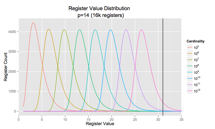
The distributions above come from the LogLog paper, on page 611, right before formula 2. Look for $\mathbb{P}_{\nu}(M = k)$ .

Consider the setting in the paper where $p = \log_2(m) = 14$ . Let’s says we wanted to safely count into the 100 billion range. If we have $L = p + (2^5 - 1) = 14 + 31 = 45$ then our new “large range correction” boundary is roughly one trillion, per the adapted formula above. As you can see from the graph below, even at $p = 10, L = 41$ the large range correction only kicks in at a little under 100 billion!

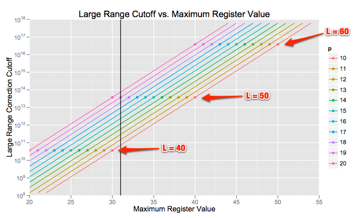
The black line is the cutoff for a 5-bit register, and the points are plotted when the total number of hash bits required reaches 40, 50, and 60.

The real question though is all this practically useful? I would argue no: there are no internet phenomena that I know of that are producing more than tens of billions of distinct values, and there’s not even a practical way of empirically testing the accuracy of HLL at cardinalities above 100 billion. (Assuming you could insert 50 million unique, random hashed values per second, it would take half an hour to fill an HLL to 100 billion elements, and then you’d have to repeat that 5000 times as they do in the paper for a grand total of 4 months of compute time per cardinality in the range.)

[UPDATE: After talking with Marc Nunkesser (one of the authors) it seems that Google may have a legitimate need for both the 100 billion to trillion range right now, and even more later, so I retract my statement! For the rest of us mere mortals, maybe this section will be useful for picking whether or not you need five or six bits.]

At AK we’ve run a few hundred test runs at 1, 1.5, and 2 billion distinct values under the $p = 10-14, L = 41-45$ configuration range and found the relative error to be identical to that of lower cardinalities (in the millions of DVs). There’s really no reason to inflate the storage requirements for large cardinality HLLs by 20% simply because the hash space has expanded. Furthermore, you can do all kinds of simple tricks like storing an offset as metadata (which would only require at most 5 bits) for a whole HLL and storing the register values as the difference from that base offset, in order to make use of a larger hash space.

Small Cardinality Estimation

Simply put, the paper introduces a second small range correction between the existing one (linear counting) and the “normal” harmonic mean estimator ( $E$ in the original paper) in order to eliminate the “large” jump in relative error around the boundary between the two estimators.

They empirically calculate the bias of $E$ and create a lookup table for various $p$ , for 200 values less than $5 \cdot 2^p$ with a correction to the overestimate of $E$ . They interpolate between the 200 reference points to determine the correction to apply for any given raw $E$ value. Their plots give compelling evidence that this bias correction makes a difference in the $m$ to $5m$ cardinality range (cuts 95th percentile relative error from about 2% to 1.2%).

I’ve been a bit terse about this improvement since sadly it doesn’t help us at AK much because most of our data is Zipfian. Few of our reporting keys live in the narrow cardinality range they are optimizing: they either wallow in the linear counting range or shoot straight up into the normal estimator range.

Nonetheless, if you find you’re doing a lot of DV counting in this range, these corrections are pretty cheap to implement (as they’ve provided numerical values for all the cutoffs and bias corrections in the appendix.)

Sparse representation

The general theme of this optimization isn’t particularly new (our friends at MetaMarkets mentioned it in this post): for smaller cardinality HLLs there’s no need to materialize all the registers. You can get away with just materializing the set registers in a map. The paper proposes a sorted map (by register index) with a hash map off the side to allow for fast insertions. Once the hash map reaches a certain size, its entries are batch-merged into the sorted list, and once the sorted list reaches the size of the materialized HLL, the whole thing is converted to the fully-materialized representation.

Aside: Though the hash map is a clever optimization, you could skip it if you didn’t want the added complexity. We’ve found that the simple sorted list version is extremely fast (hundreds of thousands of inserts per second). Also beware the variability of the the batched sort-and-merge cost every time the hash map repeatedly outgrows its limits and has to be merged into the sorted list. This can add significant latency spikes to a streaming system, whereas a one-by-one insertion sort to a sorted list will be slower but less variable.

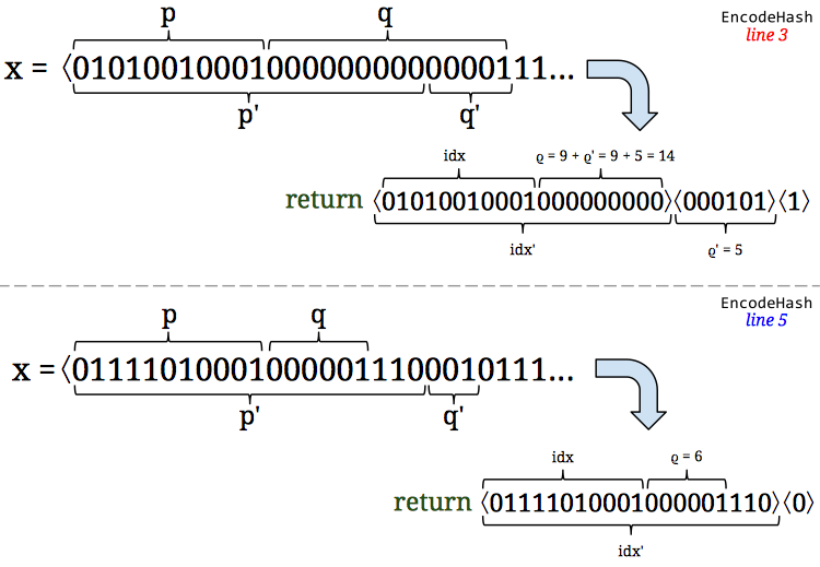
The next bit is very clever: they increase $p$ when the HLL is in the sparse representation because of the saved space. Since they’re already storing entries in 32-bit integers, they increase $p$ to $p^{\prime} = 31 - \mbox{regWidth} = 31 - 6 = 25$ . (I’ll get to the leftover bit in a second!) This gives them increased precision which they can simply “fold” down when converting from the sparse to fully materialized representation. Even more clever is their trick of not having to always store the full register value as the value of an entry in the map. Instead, if the longer register index encodes enough bits to determine the value, they use the leftover bit I mentioned before to signal as much.

In the diagram, $p$ and $p^{\prime}$ are as in the Google paper, and $q$ and $q^{\prime}$ are the number of bits that need to be examined to determine $\rho$ for either the $p$ or $p^{\prime}$ regime. I encourage you to read section 5.3.3 as well as EncodeHash and DecodeHash in Figure 8 to see the whole thing. [UPDATE: removed the typo section as it has been fixed in the most recent version of the paper (linked at the top)]

The paper also tacks on a difference encoding (which works very well because it’s a sorted list) and a variable length encoding to the sparse representation to further shrink the storage needed, so that the HLL can use the increased register count, $p^{\prime}$ , for longer before reverting to the fully materialized representation at $p$ . There’s not much to say about it because it seems to work very well, based on their plots, but I’ll note that in no way is that type of encoding suitable for streaming or “real-time” applications. The encode/decode overhead simply takes an already slow (relative to the fully materialized representation) sparse format and adds more CPU overhead.

Conclusion

The researchers at Google have done a great job with this paper, meaningfully tackling some hard engineering problems and showing some real cleverness. Most of the optimizations proposed work very well in a database context, where the HLLs are either being used as temporary aggregators or are being stored as read-only data, however some of the optimizations aren’t suitable for streaming/”real-time” work. On a more personal note, it’s very refreshing to see real algorithmic engineering work being published from industry. Rob, Matt, and I just got back from New Orleans and SODA / ALENEX / ANALCO and were hoping to see more work in this area, and Google sure did deliver!

Appendix

Sebastiano Vigna brought up the point that 6-bit registers are necessary for counting above 4 billion in the comments. I addressed it in the original post (see “A solution and a rebuttal“) but I’ll lay out the math in a bit more detail here to show that you can easily count above 4 billion with only 5-bit registers.

If you examine the original LogLog paper (the same as mentioned above) you’ll see that the register distribution for LogLog (and HyperLogLog consequently) registers is

$\displaystyle \mathbb{P}_{\nu}(M > k) = 1 - \mathbb{P}_{\nu}(M \le k) = 1 - \Big(1 - \frac{1}{2^k}\Big)^{\nu}$

where $k$ is the register value and $\nu$ is the number of (distinct) elements a register has seen.

So, I assert that 5 bits for a register (which allows the maximum value to be 31) is enough to count to ten billion without any special tricks. Let’s fix $p=14$ and say we insert $10^{10}$ distinct elements. That means, any given register will see about $\frac{10^{10}}{2^p} = \frac{10^{10}}{2^{14}} = \approx 6.1 \times 10^5$ elements assuming we have a decent hash function. So, the probability that a given register will have a value greater than 31 is (per the LogLog formula given above)

$\displaystyle \mathbb{P}_{\nu}(M > 31) = 1 - \mathbb{P}_{\nu}(M \le 31) = 1 - \Big(1 - \frac{1}{2^{31}}\Big)^{6.1 \times 10^5} \approx 0.00028$

and hence the expected number of registers that would overflow is approximately $2^{14} \times 0.00028 \approx 4.5$ . So five registers out of sixteen thousand would overflow. I am skeptical that this would meaningfully affect the cardinality computation. In fact, I ran a few tests to verify this and found that the average number of registers with values greater than 31 was 4.5 and the relative error had the same standard deviation as that predicted by the paper, $1.04/\sqrt{m}$ .

For argument, let’s assume that you find those five overflowed registers to be unacceptable. I argue that you could maintain an offset in 5 bits for the whole HLL that would allow you to still use 5 bit registers but exactly store the value of every register with extremely high probability. I claim that with overwhelmingly high probability, every register the HLL used above is greater than 15 and less than or equal to 40. Again, we can use the same distribution as above and we find that the probability of a given register being outside those bounds is

$\mathbb{P}_{\nu}(M < 15) \approx 10^{-162}$ and

$\mathbb{P}_{\nu}(M > 40) \approx 10^{-7}$ .

Effectively, there are no register values outside of $[15,40]$ . Now I know that I can just store 15 in my offset and the true value minus the offset (which now fits in 5 bits) in the actual registers.

Comments

Matt Abrams says:

January 24, 2013 at 12:58 pm

Great points on the 6 bit register and the CPU overhead of the encoding. I’m still working on my implementation but I think I’ll offer some parameters to turn the level of encoding up and down. None, just varint encoding, varint+delta encoding. The authors of the paper have posted a updated version that has a few minor corrections. I haven’t found it on the web yet but it should be there soon.

For anyone who is interested here is my attempt (far from complete) to implement this algorithm. https://github.com/clearspring/stream-lib/blob/hll_plus_plus/src/main/java/com/clearspring/analytics/stream/cardinality/HyperLogLogPlus.java

- timonk says:
  
  January 24, 2013 at 1:24 pm
  
  Thanks, Matt! Looking forward to seeing what kind of performance differences you see with the different encoding options.
  
Sebastiano Vigna says:

January 25, 2013 at 3:18 pm

We have actually been using 64-bit HyperLogLog counter since a while. That’s how we measured Facebook’s “degree of separation” in 2011 (http://arxiv.org/abs/1111.4570). It actually made the NYT! (http://www.nytimes.com/2011/11/22/technology/between-you-and-me-4-74-degrees.html). 6 bits are necessary for more than 4 billion entries—the HyperLogLog bounds from the original papers are really tight. In our code we use exactly the ceiling of log log n as number of bits per register.

- timonk says:
  
  January 29, 2013 at 12:04 pm
  
  Hi Sebastiano,
  
  Glad to see HyperLogLog is getting use in all kinds of different settings! The paper was a very interesting read, thanks! I’ve responded at the bottom of the post to address the five versus six bit registers so I could use the nice latex formatting. Please take a look!
  
  Thanks,
  Timon
  
Metin Döşlü says:

March 11, 2013 at 8:52 am

Hey Timon,

Given the experimental results on the paper, have you ever considered using Linear Counting until threshold 5m instead of 5m/2 ?

Thanks,
Metin

- timonk says:
  
  March 11, 2013 at 12:41 pm
  
  Hi Metin,
  
  We had given it some thought but found (like the paper) that Linear Counting is only competitive until about 7/2 * m, after which the raw estimator works better. Like I mentioned in the post, we’re not terribly interested in the (5/2 * m to 7/2 * m) range so we haven’t bothered to change anything in our implementation.
  
  -Timon
  
milvakili says:

July 2, 2013 at 10:44 pm

I do not understand what keep us using 64/128 bit hash in the case of HLL? or why the original paper uses 32 bit by default and HLL+ uses 64 bit? What is the main difference between HLL+ and HLL with 64 bit hash? Aside from the sparsity.

- timonk says:
  
  September 25, 2013 at 2:12 pm
  
  The original used 32 bits by default probably because that was the common machine word size and non-cryptographic hash output size at the time of research and publishing. The differences between an adapted 64-bit HLL and HLL++, if we ignore the sparse representation trick, are simply the small-range cardinality correction and a move to 6-bit registers.

HyperLogLog++: Google’s Take On Engineering HLL

32-bit vs. 64-bit hash function

Some math

A solution and a rebuttal

Small Cardinality Estimation

Sparse representation

Conclusion

Appendix

Comments

Trackbacks

Leave a comment Cancel reply

HyperLogLog++: Google’s Take On Engineering HLL

32-bit vs. 64-bit hash function

Some math

A solution and a rebuttal

Small Cardinality Estimation

Sparse representation

Conclusion

Appendix

Share this:

Related

Comments

Trackbacks

Leave a comment Cancel reply