Hitting the Books: EADS Summer School on Hashing

Rob, Matt, and I just wrapped up our trip to Copenhagen for the EADS Summer School on Hashing at the University of Copenhagen and it was a blast! The lineup of speakers was, simply put, unbeatable: Rasmus Pagh, Graham Cormode, Michael Mitzenmacher, Mikkel Thorup, Alex Andoni, Haim Kaplan, John Langford, and Suresh Venkatasubramanian. There’s a good chance that any paper you’ve read on hashing, sketching, or streaming has one of them as a co-author or is heavily influenced by their work. The format was three hour-and-a-half lectures for four days, with exercises presented at the end of each lecture. (Slides can be found here. They might also post videos. UPDATE: They’ve posted videos!)

Despite the depth of the material, almost all of it was approachable with some experience in undergraduate math and computer science. We would strongly recommend both of Michael Mitzenmacher’s talks (1, 2) for an excellent overview of Bloom Filters and Cuckoo hashing that are, in my opinion, significantly better and more in depth than any other out there. Specifically, the Bloom Filter talk presents very elegantly the continuum of Bloom Filter to Counting Bloom Filter to Count-Min Sketch (with “conservative update”) to the Stragglers Problem and Invertible Bloom Filters to, finally, extremely recent work called Odd Sketches.

Similarly, Mikkel Thorup’s two talks on hashing (1, 2) do a very thorough job of examining the hows and whys of integer hashing, all the way from the simplest multiply-mod-prime schemes all the way to modern work on tabulation hashing. And if you haven’t heard of tabulation hashing, and specifically twisted tabulation hashing, get on that because (1) it’s amazing that it doesn’t produce trash given how simple it is, (2) it’s unbelievably fast, and (3) it has been proven to provide the guarantees required for almost all of the interesting topics we’ve discussed on the blog in the past: Bloom Filters, Count-Min sketch, HyperLogLog, chaining/linear-probing/cuckoo hash tables, and so on. We really appreciated how much attention Mikkel devoted to practicality of implementation and to empirical performance when discussing hashing algorithms. It warms our heart to hear a leading academic in this field tout the number of nanoseconds it takes to hash an item as vocally as the elegance of the proof behind it!

We love this “Summer School” format because it delivers the accumulated didactic insight of the field’s top researchers and educators to both old techniques and brand new ones. (And we hope by now that everyone reading our blog appreciates how obsessed we are with teaching and clarifying interesting algorithms and data structures!) Usually most of this insight (into origins, creative process, stumbling blocks, intermediate results, inspiration, etc.) only comes out in conversation or lectures, and even worse is withheld or elided at publishing time for the sake of “clarity” or “elegance”, which is a baffling rationale given how useful these “notes in the margin” have been to us. The longer format of the lectures really allowed for useful “digressions” into the history or inspiration for topics or proofs, which is a huge contrast to the 10-minute presentations given at a conference like SODA. (Yes, obviously the objective of SODA is to show a much greater breadth of work, but it really makes it hard to explain or digest the context of new work.)

In much the same way, the length of the program really gave us the opportunity to have great conversations with the speakers and attendees between sessions and over dinner. We can’t emphasize this enough: if your ambition to is implement and understand cutting edge algorithms and data structures then the best bang for your buck is to get out there and meet the researchers in person. We’re incredibly lucky to call most of the speakers our friends and to regularly trade notes and get pointers to new research. They have helped us time and again when we’ve been baffled by inconsistent terminology or had a hunch that two pieces of research were “basically saying the same thing”. Unsurprisingly, they are also the best group of people to talk to when it comes to understanding how to foster a culture of successful research. For instance, Mikkel has a great article on how to systematically encourage and reward research article that appears in the March 2013 issue of CACM (pay-wall’d). Also worthwhile is his guest post on Bertrand Meyer’s blog.

If Mikkel decides to host another one of these, we cannot recommend attending enough. (Did we mention it was free?!) Thanks again Mikkel, Rasmus, Graham, Alex, Michael, Haim, and John for organizing such a great program and lecturing so eloquently!

Open Source Release: js-murmur3-128

As you can imagine from of all of our blog posts about hashing that we hash a lot of things. While the various hashing algorithms may be well-defined, the devil is always in the details especially when working with multiple languages that have different ways of representing numbers. We’re happy to announce the open-source release of AK’s 128bit Murmur3 implementation for JavaScript, js-murmur3-128. We are releasing this code under the Apache License, Version 2.0 matching our other open source offerings.

Details

The goal of the implementation is to produce a hash value that is equivalent to the C++ and Java (Guava) versions for the same input and it must be usable in the browser. (Full disclosure: we’re still working through some signed/unsigned issues between the C++ and Java/JavaScript versions. The Java and JavaScript versions match exactly.)

Usage

Java (Guava):

final int seed = 0;
final byte[] bytes = { (byte)0xDE, (byte)0xAD, (byte)0xBE, (byte)0xEF,
                       (byte)0xFE, (byte)0xED, (byte)0xFA, (byte)0xCE };
com.google.common.hash.HashFunction hashFunction = com.google.common.hash.Hashing.murmur3_128(seed);
com.google.common.hash.HashCode hashCode = hashFunction.newHasher()
       .putBytes(bytes)
       .hash();
System.err.println(hashCode.asLong());

JavaScript:

var seed = 0;
var rawKey = new ArrayBuffer(8);
    var byteView = new Int8Array(rawKey);
        byteView[0] = 0xDE; byteView[1] = 0xAD; byteView[2] = 0xBE; byteView[3] = 0xEF;
        byteView[4] = 0xFE; byteView[5] = 0xED; byteView[6] = 0xFA; byteView[7] = 0xCE;
console.log(murmur3.hash128(rawKey, seed));

Open Source Release: postgresql-hll

We’re happy to announce the first open-source release of AK’s PostgreSQL extension for building and manipulating HyperLogLog data structures in SQL, postgresql-hll. We are releasing this code under the Apache License, Version 2.0 which we feel is an excellent balance between permissive usage and liability limitation.

What is it and what can I do with it?

The extension introduces a new data type, hll, which represents a probabilistic distinct value counter that is a hybrid between a HyperLogLog data structure (for large cardinalities) and a simple set (for small cardinalities). These structures support the basic HLL methods: insert, union, and cardinality, and we’ve also provided aggregate and debugging functions that make using and understanding these things a breeze. We’ve also included a way to do schema versioning of the binary representations of hlls, which should allow a clear path to upgrading the algorithm, as new engineering insights come up.

A quick overview of what’s included in the release:

  • C-based extension that provides the hll data structure and algorithms
  • Austin Appleby’s MurmurHash3 implementation and SQL-land wrappers for integer numerics, bytes, and text
  • Full storage specification in STORAGE.markdown
  • Full function reference in REFERENCE.markdown
  • .spec file for rpmbuild
  • Full test suite

A quick note on why we included MurmurHash3 in the extension: we’ve done a good bit of research on the importance of a good hash function when using sketching algorithms like HyperLogLog and we came to the conclusion that it wouldn’t be very user-friendly to force the user to figure out how to get a good hash function into SQL-land. Sure, there are plenty of cryptographic hash functions available, but those are (computationally) overkill for what is needed. We did the research and found MurmurHash3 to be an excellent non-cryptographic hash function in both theory and practice. We’ve been using it in production for a while now with excellent results. As mentioned in the README, it’s of crucial importance to reliably hash the inputs to hlls.

Why did you build it?

The short answer is to power these two UIs:

On the left is a simple plot of the number of unique users seen per day and the number of cumulative unique users seen over the days in the month. The SQL behind this is very very straightforward:

SELECT report_date,
       #users as by_day,
       #hll_union_agg(users) as cumulative_by_day OVER (ORDER BY report_date ASC)
FROM daily_uniques
WHERE report_date BETWEEN '2013-01-01' AND '2013-01-31'
ORDER BY report_date ASC;

where daily_uniques is basically:

   Column    | Type | Modifiers 
-------------+------+-----------
 report_date | date | 
 users       | hll  |

Briefly, # is the cardinality operator which is operating on the hll result of the hll_union_agg aggregate function which unions the previous days’ hlls.

On the right is a heatmap of the percentage of an inventory provider’s users that overlap with another inventory provider. Essentially, we’re doing interactive set-intersection of operands with millions or billions of entries in milliseconds. This is intersection computed using the inclusion-exclusion principle as applied to hlls:

SELECT ip1.id as provider1,
       ip2.id as provider2,
       (#ip1.users + #ip2.users - #hll_union(ip1.users, ip2.users))/#ip1.users as overlap
FROM inventory_provider_stats ip1, inventory_provider_stats ip2
WHERE ip1.id <> ip2.id;

where inventory_provider_stats is basically:

   Column    | Type | Modifiers 
-------------+------+-----------
 id          | date | 
 users       | hll  |

(Some of you may note that the diagonal is labeled “exclusive reach” and is not represented in the query’s result set. That’s because the SQL above is a simplification of what’s happening. There’s some extra work done that replaces that the useless diagonal entries with the percent of the inventory provider’s users that are only seen on that inventory provider.)

We’ve been running this type of code in production for over a year now and are extremely pleased with its performance, ease of use, and expressiveness. Everyone from engineers to researchers to ops people to analysts have been using hlls in their daily reports and queries. We’re seeing product innovation coming from all different directions in the organization as a direct result of having these powerful data structures in an easily accessed and queried format. Dynamic COUNT(DISTINCT ...) queries that would have taken minutes or hours to compute from a fact table or would have been impossible in traditional cube aggregates return in milliseconds. Combine that speed with PostgreSQL’s window and aggregate functions and you have the ability to present interactive, rich distinct-value reporting over huge data sets. I’ll point you to the README and our blog posts on HyperLogLog for more technical details on storage, accuracy, and in-depth use cases.

I believe that this pattern of in-database probabilistic sketching is the future of interactive analytics. As our VP of Engineering Steve Linde said to me, “I can’t emphasize enough how much business value [sketches] deliver day in and day out.”

Our Commitment

Obviously we’re open-sourcing this for both philanthropic and selfish reasons: we’d love for more people to use this technology so that they can tell us all the neat uses for it that we haven’t thought of yet. In exchange for their insight, we’re promising to stay active in terms of stewardship and contribution of our own improvements. Our primary tool for this will be the GitHub Issues/Pull Request mechanism. We’d considered a mailing list but that seems like overkill right now. If people love postgresql-hll, we’ll figure something out as needed.

Please feel free to get in touch with us about the code on GitHub and about the project in general in the comments here. We hope to release additional tools that allow seamless Java application integration with the raw hll data in the future, so stay tuned!


Update

Looks Dimitri Fontaine wrote up a basic “how-to” post on using postgresql-hll here and another on unions here. (Thanks, Dimitri!) He brings up the issue that hll_add_agg() returns NULL when aggregating over an empty set when it should probably return an empty hll. Hopefully we’ll have a fix for that soon. You can follow the progress of the issue here.

HyperLogLog++: Google’s Take On Engineering HLL

Matt Abrams recently pointed me to Google’s excellent paper “HyperLogLog in Practice: Algorithmic Engineering of a State of The Art Cardinality Estimation Algorithm” [UPDATE: changed the link to the paper version without typos] and I thought I’d share my take on it and explain a few points that I had trouble getting through the first time. The paper offers a few interesting improvements that are worth noting:

  1. Move to a 64-bit hash function
  2. A new small-cardinality estimation regime
  3. A sparse representation

I’ll take a look at these one at a time and share our experience with similar optimizations we’ve developed for a streaming (low latency, high throughput) environment.

32-bit vs. 64-bit hash function

I’ll motivate the move to a 64-bit hash function in the context of the original paper a bit more since the Google paper doesn’t really cover it except to note that they wanted to count billions of distinct values.

Some math

In the original HLL paper, a 32-bit hash function is required with the caveat that measuring cardinalities in the hundreds of millions or billions would become problematic because of hash collisions. Specifically, Flajolet et al. propose a “large range correction” for when the estimate E is greater than 2^{32}/30.  In this regime, they replace the usual HLL estimate by the estimate

\displaystyle E^* := -2^{32} \mbox{log}\Big(1 - \frac{E}{2^{32}}\Big).

This reduces to a simple probabilistic argument that can be modeled with balls being dropped into bins. Say we have an L-bit hash. Each distinct value is a ball and each bin is designated by a value in the hash space.  Hence, you “randomly” drop a ball into a bin if the hashed value of the ball corresponds to the hash value attached to the bin.  Then, if we get an estimate E for the cardinality, that means that (approximately) E of our bins have values in them, and so there are 2^L - E empty bins.  The number of empty bins should be about 2^L e^{ - n/2^{L} }, where n is the number of balls.  Hence 2^{L} - E = 2^{L} e^{-n/2^{L}}.  Solving this gives us the formula he recommends using: -2^L \log(1 - \frac{E}{2^{L}}).

Aside:  The empty bins expected value comes from the fact that

E(\# \text{ of empty bins}) = m(1 - \frac{1}{m})^{n},

where m is the number of bins and n the number of balls.  This is pretty quick to show by induction.  Hence,

\displaystyle E(\#\text{ of empty bins}) \sim m e^{-n/m} as n \rightarrow \infty.

Again, the general idea is that the E ends up being some number smaller than n because some of the balls are getting hashed to the same value.  The correction essentially doesn’t do anything in the case when E is small compared to 2^L as you can see here. (Plotted is -\log(1 - x), where x represents E / 2^L, against the line y = x. The difference between the two graphs represents the difference between
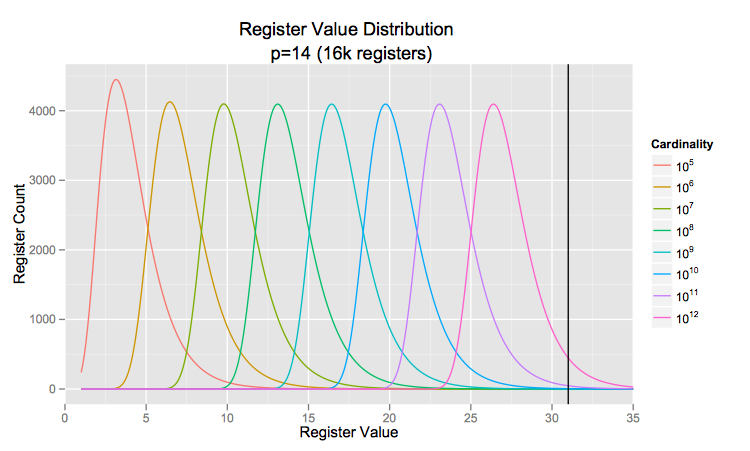
 E and n.)

A solution and a rebuttal

The natural move to start estimating cardinalities in the billions is to simply move to a larger hash space where the hash collision probability becomes negligibly small. This is fairly straightforward since most good hash functions give you at least 64-bits of entropy these days and it’s also the size of a machine word. There’s really no downside to moving to the larger hash space, from an engineering perspective. However, the Google researchers go one step further: they increase the register width by one bit (to 6), as well, ostensibly to be able to support the higher possible register values in the 64-bit setting. I contend this is unnecessary. If we look at the distribution of register values for a given cardinality, we see that it takes about a trillion elements before a 5-bit register overflows (at the black line):

regdistro-1

The distributions above come from the LogLog paper, on page 611, right before formula 2. Look for \mathbb{P}_{\nu}(M = k).

Consider the setting in the paper where p = \log_2(m) = 14. Let’s says we wanted to safely count into the 100 billion range. If we have L = p + (2^5 - 1) = 14 + 31 = 45 then our new “large range correction” boundary is roughly one trillion, per the adapted formula above. As you can see from the graph below, even at p = 10, L = 41 the large range correction only kicks in at a little under 100 billion!

lrcvsmrv-2

The black line is the cutoff for a 5-bit register, and the points are plotted when the total number of hash bits required reaches 40, 50, and 60.

The real question though is all this practically useful? I would argue no: there are no internet phenomena that I know of that are producing more than tens of billions of distinct values, and there’s not even a practical way of empirically testing the accuracy of HLL at cardinalities above 100 billion. (Assuming you could insert 50 million unique, random hashed values per second, it would take half an hour to fill an HLL to 100 billion elements, and then you’d have to repeat that 5000 times as they do in the paper for a grand total of 4 months of compute time per cardinality in the range.)

[UPDATE: After talking with Marc Nunkesser (one of the authors) it seems that Google may have a legitimate need for both the 100 billion to trillion range right now, and even more later, so I retract my statement! For the rest of us mere mortals, maybe this section will be useful for picking whether or not you need five or six bits.]

At AK we’ve run a few hundred test runs at 1, 1.5, and 2 billion distinct values under the p = 10-14, L = 41-45 
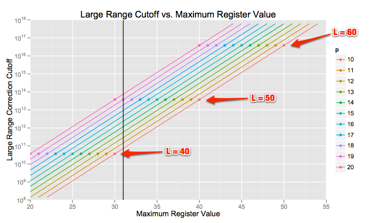
configuration range and found the relative error to be identical to that of lower cardinalities (in the millions of DVs). There’s really no reason to inflate the storage requirements for large cardinality HLLs by 20% simply because the hash space has expanded. Furthermore, you can do all kinds of simple tricks like storing an offset as metadata (which would only require at most 5 bits) for a whole HLL and storing the register values as the difference from that base offset, in order to make use of a larger hash space.

Small Cardinality Estimation

Simply put, the paper introduces a second small range correction between the existing one (linear counting) and the “normal” harmonic mean estimator (E in the original paper) in order to eliminate the “large” jump in relative error around the boundary between the two estimators.

They empirically calculate the bias of E and create a lookup table for various p, for 200 values less than 5 \cdot 2^p with a correction to the overestimate of E. They interpolate between the 200 reference points to determine the correction to apply for any given raw E value. Their plots give compelling evidence that this bias correction makes a difference in the m to 5m cardinality range (cuts 95th percentile relative error from about 2% to 1.2%).

I’ve been a bit terse about this improvement since sadly it doesn’t help us at AK much because most of our data is Zipfian. Few of our reporting keys live in the narrow cardinality range they are optimizing: they either wallow in the linear counting range or shoot straight up into the normal estimator range.

Nonetheless, if you find you’re doing a lot of DV counting in this range, these corrections are pretty cheap to implement (as they’ve provided numerical values for all the cutoffs and bias corrections in the appendix.)

Sparse representation

The general theme of this optimization isn’t particularly new (our friends at MetaMarkets mentioned it in this post): for smaller cardinality HLLs there’s no need to materialize all the registers. You can get away with just materializing the set registers in a map. The paper proposes a sorted map (by register index) with a hash map off the side to allow for fast insertions. Once the hash map reaches a certain size, its entries are batch-merged into the sorted list, and once the sorted list reaches the size of the materialized HLL, the whole thing is converted to the fully-materialized representation.

Aside: Though the hash map is a clever optimization, you could skip it if you didn’t want the added complexity. We’ve found that the simple sorted list version is extremely fast (hundreds of thousands of inserts per second). Also beware the variability of the the batched sort-and-merge cost every time the hash map repeatedly outgrows its limits and has to be merged into the sorted list. This can add significant latency spikes to a streaming system, whereas a one-by-one insertion sort to a sorted list will be slower but less variable.

The next bit is very clever: they increase p when the HLL is in the sparse representation because of the saved space. Since they’re already storing entries in 32-bit integers, they increase p to p^{\prime} = 31 - \mbox{regWidth} = 31 - 6 = 25. (I’ll get to the leftover bit in a second!) This gives them increased precision which they can simply “fold” down when converting from the sparse to fully materialized representation. Even more clever is their trick of not having to always store the full register value as the value of an entry in the map. Instead, if the longer register index encodes enough bits to determine the value, they use the leftover bit I mentioned before to signal as much.

HLL++ sparse encoding explanation

In the diagram, p and p^{\prime} 
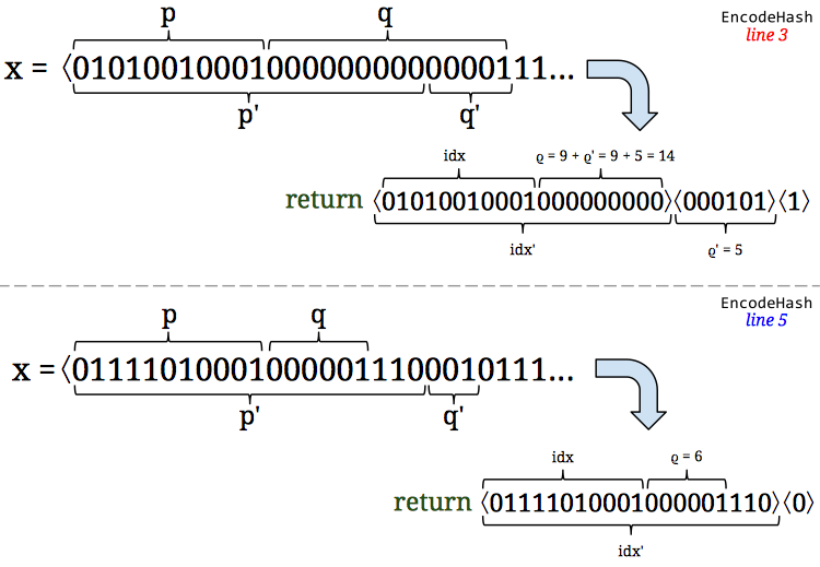
are as in the Google paper, and q and q^{\prime} are the number of bits that need to be examined to determine \rho for either the p or p^{\prime} regime. I encourage you to read section 5.3.3 as well as EncodeHash and DecodeHash in Figure 8 to see the whole thing. [UPDATE: removed the typo section as it has been fixed in the most recent version of the paper (linked at the top)]

The paper also tacks on a difference encoding (which works very well because it’s a sorted list) and a variable length encoding to the sparse representation to further shrink the storage needed, so that the HLL can use the increased register count, p^{\prime}, for longer before reverting to the fully materialized representation at p. There’s not much to say about it because it seems to work very well, based on their plots, but I’ll note that in no way is that type of encoding suitable for streaming or “real-time” applications. The encode/decode overhead simply takes an already slow (relative to the fully materialized representation) sparse format and adds more CPU overhead.

Conclusion

The researchers at Google have done a great job with this paper, meaningfully tackling some hard engineering problems and showing some real cleverness. Most of the optimizations proposed work very well in a database context, where the HLLs are either being used as temporary aggregators or are being stored as read-only data, however some of the optimizations aren’t suitable for streaming/”real-time” work. On a more personal note, it’s very refreshing to see real algorithmic engineering work being published from industry. Rob, Matt, and I just got back from New Orleans and SODA / ALENEX / ANALCO and were hoping to see more work in this area, and Google sure did deliver!


Appendix

Sebastiano Vigna brought up the point that 6-bit registers are necessary for counting above 4 billion in the comments. I addressed it in the original post (see “A solution and a rebuttal“) but I’ll lay out the math in a bit more detail here to show that you can easily count above 4 billion with only 5-bit registers.

If you examine the original LogLog paper (the same as mentioned above) you’ll see that the register distribution for LogLog (and HyperLogLog consequently) registers is

\displaystyle \mathbb{P}_{\nu}(M > k) = 1 - \mathbb{P}_{\nu}(M \le k) = 1 - \Big(1 - \frac{1}{2^k}\Big)^{\nu}

where k is the register value and \nu is the number of (distinct) elements a register has seen.

So, I assert that 5 bits for a register (which allows the maximum value to be 31) is enough to count to ten billion without any special tricks. Let’s fix p=14 and say we insert 10^{10} distinct elements. That means, any given register will see about \frac{10^{10}}{2^p} = \frac{10^{10}}{2^{14}} = \approx 6.1 \times 10^5 elements assuming we have a decent hash function. So, the probability that a given register will have a value greater than 31 is (per the LogLog formula given above)

\displaystyle \mathbb{P}_{\nu}(M > 31) = 1 - \mathbb{P}_{\nu}(M \le 31) = 1 - \Big(1 - \frac{1}{2^{31}}\Big)^{6.1 \times 10^5} \approx 0.00028

and hence the expected number of registers that would overflow is approximately 2^{14} \times 0.00028 \approx 4.5. So five registers out of sixteen thousand would overflow. I am skeptical that this would meaningfully affect the cardinality computation. In fact, I ran a few tests to verify this and found that the average number of registers with values greater than 31 was 4.5 and the relative error had the same standard deviation as that predicted by the paper, 1.04/\sqrt{m}.

For argument, let’s assume that you find those five overflowed registers to be unacceptable. I argue that you could maintain an offset in 5 bits for the whole HLL that would allow you to still use 5 bit registers but exactly store the value of every register with extremely high probability. I claim that with overwhelmingly high probability, every register the HLL used above is greater than 15 and less than or equal to 40. Again, we can use the same distribution as above and we find that the probability of a given register being outside those bounds is

\mathbb{P}_{\nu}(M < 15) \approx 10^{-162} and

\mathbb{P}_{\nu}(M > 40) \approx 10^{-7}.

Effectively, there are no register values outside of [15,40]. Now I know that I can just store 15 in my offset and the true value minus the offset (which now fits in 5 bits) in the actual registers.

K-Minimum Values: Sketching Error, Hash Functions, and You

Introduction

“All known efficient cardinality estimators rely on randomization, which is ensured by the use of hash functions.”
–Flajolet, et al

Recalling the KMV algorithm Matt presented in his last post, one will note that every stream element is passed to a hash function as part of the processing step. This is meant to transform the data being operated on from its native distribution into something uniformly distributed. Unfortunately, we don’t live in a perfect world, and since all of the algorithm’s analysis assumes that this hash function does its job well, we wanted to get some sense of how it behaves under less friendly conditions. The first half of this post will investigate the algorithm’s performance when we artificially introduce bias, and the second half will look at its behavior with a handful of real hash functions.

A Simple Error Model

The first hash function error model that came to mind is admittedly unrealistic and ham-fisted, but hopefully illustrative. Suppose you have a stream of fixed sized, an ideal hash function, and from these you produce a distinct value estimate using the KMV algorithm. Now suppose that for some unlucky reason, one bit from your hash function is stuck; it’s always a zero or a one, but the other 31 bits are free of this curse.

Biased hash schematic

There’s nothing to stop you from computing a distinct value estimate using this janky hash with KMV, but your intuition suggests that it shouldn’t be very good. We went through this exact process with various choices of k, using a random number generator to simulate a perfect hash function.

Before we look at the data, let’s think about what we should expect. From the perspective of KMV, it shouldn’t make a whole lot of difference if your kth smallest element is odd or even (for instance, in a case where the lowest order bit always/never set, respectively). It does, however, make a difference if you’re actually incapable of seeing values smaller than 231, which is what happens when the highest order bit is always set. Thus, in both the 0-biasing and 1-biasing cases, we should expect that higher order bits have a much more dramatic effect on error than lower order bits.

Error from setting bits in KMV

Notice how the performance degradation follows two different patterns. When we are fixing bits as ones, the observed error increases fairly smoothly, and tends to result in under estimates. In contrast, setting bits to zeros results in no change until the error increases producing catastrophic over estimates. Additionally, larger values of k have protective effects against these biases.

A Somewhat Less Simple Error Model

Now that we have some intuition for the problem, let’s get a little more subtle. Instead of always setting the nth bit as a 0 or 1, let’s add a probabilistic element. We’ll do the same experiment as before, except we will now fix the nth bit with probability p. Thus, when p = 0 we have a perfectly well behaved KMV, and when p = 1, we have the experiment we just finished discussing. In the following diagram, each tile represents the average error across several experiments in which a stream of 1,000,000 unique elements was fed to a KMV sketch (k = 1024) which was rigged to modify the nth bit with probability p.

Heatmap of KMV error

Many of the same lessons can be seen here — high order bits matter more, downward biasing degrades performance sharply, upward biasing degrades more smoothly. Additionally, as we’d expect, within a given bit, more bias means more error.

Send in the Hash Functions

All of the experiments to this point have involved using a random number generator instead of hashing real data. I think it’s time that we took a look at what happens when we drop in a few real hash functions with real data. For the following experiments, I’m using four 32-bit hashes — Murmur3, SDBM, Arash Partow’s hash, and one of the old Donald Knuth hashes. You may recall these from our series on choosing a good hash function (although 64-bit versions were used there). I chose four text corpuses:

  • Romeo and Juliet, stripped of all punctuation and converted to lower case (3794 words)
  • /usr/share/dict/words (99171 words)
  • 1,000,000 random 12 character long strings, each sharing the same suffix: “123456”
  • 1,000,000 random 12 character long strings, each sharing the same prefix: “123456”

Using formulas from this paper, we can compute the relative error that 99% of KMV estimates should theoretically fall within. This turns out to depend on k and the stream size.

To make these pictures, I chose random values of k within each hash/document pair at which I evaluate the cardinality estimate and compute the relative error. The lines are linear interpolations between sampled points and are shown solely for clarity. The y-axis scale is adjusted on a per-picture basis to best display the theoretical envelope within which we expect our errors to lie.

Now that we’ve gotten through all the necessary preamble, let’s take a look at the results!

KMV error for Romeo and Juliet

One picture in and we’ve already learned a lesson: choice of hash function seriously matters! SDBM and DEK cause the algorithm to perform well below its capabilities. DEK’s error is actually off the charts for most of this graph, which is why it does not appear until k > 3,000.

KMV error for /usr/bin/dict/words

On a bigger corpus with tighter theoretical error bounds, Murmur3 and AP are still doing quite well. Do note, however, that AP dips outside the envelope for a while at k = 70,000 or so.

KMV error for suffixKMV error for shared-prefix strings

With the random strings, SDBM performs much better than it did on English words. DEK, however, is still hopeless. It’s a little tough to see on these pictures, but at high k, AP starts to fall off the wagon, and even Murmur3 dips outside the envelope, though not beyond what we’d expect, statistically speaking. Honestly, I was hoping for some fireworks here, but they didn’t materialize. I was wondering if we might see some hashes break on one version of these strings, and do fine on the other due to the location of the varying key bits (high order/low order). Sadly, that didn’t happen, but a negative result is a result none the less.

To summarize these, I made the following table, which shows us the percentage of time that an one of the samples falls outside the theoretical envelope. In this view, Murmur3’s superiority is clear.

AP DEK Murmur3 SDBM
Romeo and Juliet 0.00% 100.00% 0.00% 61.54%
/usr/share/dict/words
10.76% 100.00% 0.00% 68.46%
Common Suffix 7.22% 99.11% 1.10% 0.27%
Common Prefix 3.33% 100.00% 0.22% 0.0001%

Fin

KMV is a very nice little algorithm that is incredibly simple to understand, implement, and use. That said, if you’re going to make use of it, you really do need to practice some due diligence when choosing your hash function. With packages like smhasher available, trying out multiple hash functions is a cinch, and a little legwork at the start of a project can save you from confusion and despair later on!

Choosing a Good Hash Function, Part 3

Author’s note: Part three of a series studying hash functions. My last post identified a few candidate algorithms that are subjected to further scrutiny here today.

The Story So Far

The simplest attribute on which one could imagine differentiating candidate hash functions is the number of collision produced when hashing a fixed pool of keys. By that standard, my last post identified Murmur3, Jenkins, City, Spooky, FNV1/1a, SDBM, AP, and RS as possible contenders. Today we’re going to see how they compare  to each other on some more rigorous tests.

Random Uniformity

A hash function ought to distribute its keys uniformly across its output range. To see how these functions stack up, we’ll put our 42 million unique keys through each hash function, bin the output, and compare the bin counts with expectation:

For bins of equal size, E[bini] = Number of items hashed/Number of bins

Now, uniformity is different from random uniformity. In general the latter is not always necessary for building a good hash table, but the analysis of some schemes assume it. For our purposes, we’re going to want our hashes to look like they are drawn from a random uniform distribution — simple uniformity won’t cut it for our applications. This means that when we look at our bin counts, we want them to be neither too smooth nor too lumpy. To quantify this concept, we’ll use a chi-squared test.

In volume II of TAOCP Donald Knuth provides a somewhat ad-hoc, but easy to understand method for interpreting the p-values calculated by a chi-squared test of randomness. If your p-value is less than 0.01 or greater than 0.99 the process that generated those results is almost certainly non-random. Something less than 0.05 or greater than 0.95 should be considered suspect. Finally, he designates a p-value of less than 0.1 or greater than 0.90 as “almost suspect”.

Here I’ve cut the whole 64 bit output space into 100 bins, and again in 1,000,000 bins. For a final test I modded out the bottom 20 bits, to check their distributions in isolation.

Hash Function 1 Million bins* Bottom 20 bits* 100 bins
AP  0.70  0.50  <0.01
City 0.07  0.29  0.46
FNV64-1  <0.01  >0.99  0.97
FNV64-1a  >0.99  >0.99  0.87
Jenkins  0.17  0.46  0.72
Murmur3  0.14  0.31  0.08
RS  >0.99  >0.99  0.23
SDBM  >0.99  >0.99  >0.99
Spooky  0.84  0.27  0.98

*p-values estimated from a standard normal distribution

Jenkins passes all three of these nicely. City and Murmur each come up “almost suspect” once, and Spooky shows some suspicious behavior in the 100 bin test. I put the heaviest weight on the bottom 20 bit test, and can pretty comfortably give these four functions a pass here. AP does dramatically better at higher bin counts, which is interesting. We can pretty solidly eliminate RS, SDBM, AP, and both FNV variants based on this analysis alone.

As a final note, hash functions are not meant to be RNGs! This test holds them to a very rigid standard that is not generally necessary to build a good hash table. It’s just that in our specific application, we’re going to want our hash values to be somewhat random looking.

Using Keyspace Structure

Before I continue, let me explain a little bit more of the structure of the data I am working with. I have 251 namespaces, each of which has a variable number of 192 and 256 bit keys associated with it. All told I have in the neighborhood of 66 million datapoints of the form (namespace, key). Only the key portion of these tuples actually gets hashed, however. Up until this point, we have been ignoring the namespace attribute of these data points, and thus have been restricted to looking at the 42 million unique (key, hash(key)) pairs. Let’s see if we can exploit larger set of data by including the namespaces!

In the chi-squared analysis above, we did our binning over the union of all namespaces. Now let’s individually bin the hash values of each namespace. All said and done, we have 251 namespaces ranging in size from a tiny handful to several million elements. This gives us 251 vectors of size 100, with

V{n,i} = Number of items of namespace n hashed to the i-th bin

For each namespace, we can compute the mean and variance of its count vector. I’ll leave it as an exercise to the reader, but it’s a pretty simple calculation to show that if you sample from a random uniform distribution, the variance of such a bin-count vector should equal its mean. If the variance is lower than the mean, it implies that the distribution is flatter than expected. On the contrary, if the variance is higher, it implies the existence of hot-spots on the range that are getting more than their fair share of data points hashed there.

Enough with the words, let’s look at the graphs! To generate these, I took the subset of namespaces that had at least 100,000 elements, of which there are 83. Each point is a namespace, and the green line shows the theoretical variance = mean relationship we’d expect from binning a random uniform distribution. Finally, I ran a Bonferroni corrected chi-squared test within each namespace. Those that come out “almost suspect” or worse are highlighted in red.

You can think of these namespaces as small experiments. Together, they help give us a picture of what the chi-squared test done on the whole dataset tells us.

A few observations:

  • Under the 100 bin chi-squared test, SDBM was flagged as being way too uniformly distributed. We can see that quite clearly here. Generally, the variance of the bin counts is quite a bit lower than the mean bin count.
  • On the other hand, AP has a comparatively high variance. This translates, again, to some bins being overly “favored” by the hash function.
  • These pictures also give us some idea of how noisy the functions are on a namespace by namespace basis. Compare Spooky and Murmur3. The residuals for all of the namespaces are quite low, and basically equal for Spooky, whereas Murmur3’s residuals show a lot more variability.

So far we’ve been taking our input sets as a given, and examining the statistical properties of the outputs. While powerful, we need not limit ourselves to these techniques. Onward to avalanche!

Avalanche Analysis

A common test of hash function performance is whether or not it achieves “avalanche.” This refers to the desireable characteristic that

P(Output bit i changes | Input bit j changes) = 0.5 for all i, j

Basically, if we keep all of the input bits the same, save for exactly 1 which we flip, we’d hope that each of our hash function’s output bits changes with probability 1/2.

I generated the following avalanche diagrams by using a random sample of 4000 keys (2000 of each type). The x-axis is the input key bit, the y axis is the output hash bit, and the color of the (x,y) tile is a measure of the bias that I/O pair has. Black indicates the desired 50% flip-probability, bright green indicates that the output bit is “stuck” and, certeris paribus, it doesn’t ever vary as a result of flipping just that input bit.

Avalanche Diagram

This test absolutely wrecks AP, SDBM, both FNV twins, and RS. Jenkins has some poor mixing in its upper bits, but that is mentioned in the implementation. It’s very small, but a slight bias can be observed in City’s lowest bits on the Creative keys. Murmur3 and Spooky are the only two functions left unscathed by this test. Given some of our algorithmic needs, this is a very slight knock against both Jenkins and City.

Conclusion

After all of this, Murmur3, Jenkins, City, and Spooky are the only functions that I’m really pleased with for our work. I’ll give a slight edge to Murmur3 and City over Jenkins due to the avalanche results, and City’s incredible speed. Spooky’s performance here is notable, but I’m a little uneasy putting it forward as a candidate for use in production, as it is still in beta. I’ll be keeping my eye on it. Based on these results it shows a lot of promise!

The next logical step is to plug some of these in to Timon’s work, and see how they serve as the keystone of our hash table!

Choosing a Good Hash Function, Part 2

Author’s note: Part two of a series in which I investigate the performance of a menagerie of hash functions on our data. In today’s episode the analysis begins in earnest with an investigation of collision rates.

Hash function designers have many tools at their disposal, but at their heart, most algorithms follow the same pattern: bytewise iteration over a key during which some internal state is mixed up with the key bits via some combination of ANDs, ORs, XORs, ADDs, shifts, magic numbers, modular arithmetic, and similar tools. As an example, consider the famous FNV hash function, which is astoundingly simple in its construction:

uint64_t fnv1_hash (void *key, int n_bytes)
{
    unsigned char *p = key;
    uint64_t h = 14695981039346656037;
    int i;
    for (i = 0; i < n_bytes; i++) {
        h = (h * 1099511628211) ^ p[i];
    }
    return h;
}

With all hash functions, the hope is that one may sufficiently mix up the input bits such that, on average, the output is uniformly distributed across its available range. If you think that designing such an algorithm sounds tricky, you’re right!

Over the years many hash functions have been developed that vary widely in quality and complexity. There are many that, despite some demonstrable theoretical flaws, have worked well in enough practical applications to have gained popularity. Other algorithms have been designed from the ground up to achieve a variety of theoretical benchmarks. To get started with this project, I spent some time looking around and came up with a list of 16 reasonably well-known functions that run a pretty wide breadth of quality from negative control to veteran. I started with the simplest test imaginable: I have ~42 million keys available, each of which are either 192 or 256 bits long. Given my entire available set of keys, what fraction can be hashed without collision?

Fraction of keys hashed without collision

A few notes about this graph:

  • All hashes are 64 bits.
  • Hashing is hard. Many of these functions do quite poorly compared to sampling from a random uniform distribution. The theoretical expectation here is that 0 keys should collide.
  • It looks like there is a significant hurdle at ~85% of the keys.
  • Although hard to see on this chart, OAT (Bob Jenkins’ less popular one-at-a-time hash) came in just under 100%. While this is a standout performance in comparison to most of the functions tested, it is still below what is expected by theory.
  • Unsurprisingly, Murmur3 and Jenkins eat this data set for lunch. They are carefully designed to work well on a broad variety of inputs, thoroughly tested, and I would have been shocked to see them fail here. They are matched by Google’s City Hash, Spooky Hash (Jenkins’ most recent project, which is still under development), FNV-1/1a, SDBM hash (also known as x65599), RS (Arash Partow‘s version of a hash function designed by Robert Sedgewick), another function of Partow’s own creation.

We’re by no means done here — we’ve simply thinned our list to a few algorithms that merit deeper exploration. The challenge now becomes distinguishing our high performers, and for that we’ll need tools a little bit more sophisticated than simple collision counts. Bring your statistics thinking cap to part 3!

Appendix: Further Reading

  • Unsurprisingly, Donald Knuth’s chapter from The Art of Computer Programming, Volume III: Sorting and Searching is an excellent piece.
  • Bob Jenkins wrote a great article in Dr. Dobb’s back in 1997 that is also a great starting place.
  • More generally, Jenkins’ own website is a treasure trove of material on the subject of hashing
  • There’s a lot of material about FNV to be had here.
  • And let’s not leave out Murmur Hash and City Hash.

Choosing a Good Hash Function, Part 1

Author’s note: Hello, reader! I’m Colin, a new data scientist on the team. This is the first in a series of posts in which I will be describing my efforts to characterize various hash functions for use here at AK. Future posts will discuss the statistical and computational properties exhibited by these algorithms on our data. Additionally, I will be tackling the problem of  trying to use the data that we have available to uncover potentially pathological input sets.

At AK, every event that we track is encoded as an n-tuple of 64-bit integers:

key component #1, key component #2, … , key component #n

This is a convenient form for summary and analysis, but obviously not optimal from a storage perspective. Internet advertising is no stranger to large numbers, but 264n is enormous. The set of keys that we will draw from this theoretical universe of keys is comparatively quite small. We find ourselves posed with a problem that looks very much like a natural fit for hashing!

A well chosen hash function, operating at the heart of solidly designed hash table could allow us a big win on both the internal storage/representation front, as well as in wild, freeing up space in client cookies, etc.

Paraphrasing Knuth, one should not choose a random hash function to generate a good hash table. As with any hashing task, there are the three classical issues to consider:

  • The size of the hash in terms of the number of bits of output needed to hit your collision (two distinct keys hashing to the same value) goals and remain within your storage constraints
  • The distributions of hashes on your input data, and the related problem of collisions
  • Computation time

Over the next several posts, I will be putting a number of hash functions through the wringer in an effort to identify a handful that perform well on our data.