Neustar at re:Invent 2014

On Thursday, Nov. 13th I was given the opportunity to speak at AWS re:Invent 2014 about the ad analytics products and platforms we’ve built on Redshift. My slides are available here along with what I said in the speaker’s notes.

I covered how to implement four classical ad tech queries:

  • Frequency – how many ads should I show each user?
  • Attribution – how much should I pay for each ad?
  • Overlap – where can I find these people for cheaper?
  • Ad-hoc – how can I empower my users to run their own custom queries?

I also discussed how to take maximum advantage of Redshift’s simple orchestration and provisioning to scale to as many workloads and platforms as your heart desires and save money in the process!

It was a pleasure, as usual, to present to a packed room and to discuss all the great things the team has been up to.

HLL talk at SFPUG

I had the pleasure of speaking at the SF PostgreSQL User Group’s meetup tonight about sketching, the history of HLL, and our implementation of HLL as a PG extension. My slides are embedded below and you can get a PDF copy here. Be sure to click the gear below to show speaker’s notes for context!

If video is made available, I’ll post an update with a link!

Hitting the Books: EADS Summer School on Hashing

Rob, Matt, and I just wrapped up our trip to Copenhagen for the EADS Summer School on Hashing at the University of Copenhagen and it was a blast! The lineup of speakers was, simply put, unbeatable: Rasmus Pagh, Graham Cormode, Michael Mitzenmacher, Mikkel Thorup, Alex Andoni, Haim Kaplan, John Langford, and Suresh Venkatasubramanian. There’s a good chance that any paper you’ve read on hashing, sketching, or streaming has one of them as a co-author or is heavily influenced by their work. The format was three hour-and-a-half lectures for four days, with exercises presented at the end of each lecture. (Slides can be found here. They might also post videos. UPDATE: They’ve posted videos!)

Despite the depth of the material, almost all of it was approachable with some experience in undergraduate math and computer science. We would strongly recommend both of Michael Mitzenmacher’s talks (1, 2) for an excellent overview of Bloom Filters and Cuckoo hashing that are, in my opinion, significantly better and more in depth than any other out there. Specifically, the Bloom Filter talk presents very elegantly the continuum of Bloom Filter to Counting Bloom Filter to Count-Min Sketch (with “conservative update”) to the Stragglers Problem and Invertible Bloom Filters to, finally, extremely recent work called Odd Sketches.

Similarly, Mikkel Thorup’s two talks on hashing (1, 2) do a very thorough job of examining the hows and whys of integer hashing, all the way from the simplest multiply-mod-prime schemes all the way to modern work on tabulation hashing. And if you haven’t heard of tabulation hashing, and specifically twisted tabulation hashing, get on that because (1) it’s amazing that it doesn’t produce trash given how simple it is, (2) it’s unbelievably fast, and (3) it has been proven to provide the guarantees required for almost all of the interesting topics we’ve discussed on the blog in the past: Bloom Filters, Count-Min sketch, HyperLogLog, chaining/linear-probing/cuckoo hash tables, and so on. We really appreciated how much attention Mikkel devoted to practicality of implementation and to empirical performance when discussing hashing algorithms. It warms our heart to hear a leading academic in this field tout the number of nanoseconds it takes to hash an item as vocally as the elegance of the proof behind it!

We love this “Summer School” format because it delivers the accumulated didactic insight of the field’s top researchers and educators to both old techniques and brand new ones. (And we hope by now that everyone reading our blog appreciates how obsessed we are with teaching and clarifying interesting algorithms and data structures!) Usually most of this insight (into origins, creative process, stumbling blocks, intermediate results, inspiration, etc.) only comes out in conversation or lectures, and even worse is withheld or elided at publishing time for the sake of “clarity” or “elegance”, which is a baffling rationale given how useful these “notes in the margin” have been to us. The longer format of the lectures really allowed for useful “digressions” into the history or inspiration for topics or proofs, which is a huge contrast to the 10-minute presentations given at a conference like SODA. (Yes, obviously the objective of SODA is to show a much greater breadth of work, but it really makes it hard to explain or digest the context of new work.)

In much the same way, the length of the program really gave us the opportunity to have great conversations with the speakers and attendees between sessions and over dinner. We can’t emphasize this enough: if your ambition to is implement and understand cutting edge algorithms and data structures then the best bang for your buck is to get out there and meet the researchers in person. We’re incredibly lucky to call most of the speakers our friends and to regularly trade notes and get pointers to new research. They have helped us time and again when we’ve been baffled by inconsistent terminology or had a hunch that two pieces of research were “basically saying the same thing”. Unsurprisingly, they are also the best group of people to talk to when it comes to understanding how to foster a culture of successful research. For instance, Mikkel has a great article on how to systematically encourage and reward research article that appears in the March 2013 issue of CACM (pay-wall’d). Also worthwhile is his guest post on Bertrand Meyer’s blog.

If Mikkel decides to host another one of these, we cannot recommend attending enough. (Did we mention it was free?!) Thanks again Mikkel, Rasmus, Graham, Alex, Michael, Haim, and John for organizing such a great program and lecturing so eloquently!

Open Source Release: java-hll

We’re happy to announce our newest open-source project, java-hll, a HyperLogLog implementation in Java that is storage-compatible with the previously released postgresql-hll and js-hll implementations. And as the rule of three dictates, we’ve also extracted the storage specification that makes them interoperable into it’s own repository. Currently, all three implementations support reading storage specification v1.0.0, while only the PostgreSQL and Java implementations fully support writing v1.0.0. We hope to bring the JS implementation up to speed, with respect to serialization, shortly.

AK at re:Invent 2013

I was given the opportunity to speak at AWS re:Invent 2013, on Wednesday, Nov. 13th, about how we extract maximum performance, across our organization, from Redshift. You can find the slides here, and my voice-over, though not identical, is mostly captured by the notes in those slides.

The talk, in brief, was about the technical features of Redshift that allow us to write, run, and maintain many thousands of lines of SQL that run over hundreds of billions of rows at a time. I stayed away from nitty-gritty details in the talk, since I only had 15 minutes, and tried to focus on high-level take-aways:

  • SQL is code, so treat it like the rest of your code. It has to be clean, factored, and documented. Use CTEs to break queries into logical chunks. Use window functions to express complex ideas succinctly.
  • Redshift is an MPP system with fast IO, fast sorting, and lots of storage. Use this to your advantage by storing multiple different sort orders of your data if you have different access patterns. Materialize shared intermediates so many queries can take advantage of them.
  • Redshift has excellent integration with S3. Use the fat pipes to cheaply materialize query intermediates for debugging. Use the one-click snapshot feature to open up experimentation with schema, data layout, and column compression. If it doesn’t work out, you revert to your old snapshot.
  • Use the operational simplicity of Redshift to be frugal. Turn over the responsibility of managing cluster lifecycles to the people that use them. For instance, devs and QA rarely need their clusters when the workday is done. The dashboards are such a no-brainer that it’s barely a burden to have them turn off and start up their own clusters. Allow users to take responsibility for their cluster, and they will become more responsible about using their cluster.
  • Use the operational simplicity of Redshift to be more aware. With just a few clicks, you can launch differently sized clusters and evaluate your reports and queries against all of them. Quantify the cost of your queries in time and money.
  • It’s a managed service: stop worrying about nodes and rows and partitions and compression! Get back to business value:
    • How long does the customer have to wait?
    • How much does this report cost?
    • How do I make my staff more productive?
    • How do I minimize my technical debt?

Slides and Videos are up for AK Data Science Summit

We’re happy to announce that all the talks (slides and video) from our Data Science Summit are available for free, right here on the blog! You can find a full list of the conference’s content here.

Enjoy!

AWS Redshift: How Amazon Changed The Game

Edit: Thank you to Curt Monash who points out that Netezza is available for as little as $20k/TB/year with hardware (and 2.25x compression) and that there is an inconsistency in my early price estimates and the fraction I quote in my conclusion. I’ve incorporated his observations into my corrections below. I’ve also changed a sentence in the conclusion to make the point that the $5k/TB/year TCO number is the effective TCO given that a Redshift cluster that can perform these queries at the desired speed has far more storage than is needed to just hold the tables for the workloads I tested.

Author’s Note: I’ll preface this post with a warning: some of the content will be inflammatory if you go into it with the mindset that I’m trying to sell you on an alternative to Hadoop. I’m not. I’m here to talk about how an MPP system blew us away, as jaded as we are, and how it is a sign of things to come. There’s enormous, ripe-for-the-picking business value in Redshift and you’d be remiss to ignore it because “we’re a Hadoop shop” or “commercial MPP is too expensive”.

Flash back a few years: We’d struggled mightily with commercial data warehouses that simply couldn’t load the data volumes we wanted to query (at that time this was significantly less than a billion rows) in any decent amount of time, let alone query them semi-interactively. Anecdotally, we’d hear that vendor X had solved our problem or vendor Y had a completely different model that would “completely blow us out of the water“, and so on, but either the prices were astronomical ($100k/TB/year +) or the performance didn’t pan out. In our minds, MPP solutions were a non-starter.

To oversimplify the design we chose for our infrastructure: we built the Summarizer and threw in some Postgres for our product reporting needs, mixed in some Elastic Map-Reduce for the “tough” jobs, and went about our business. We’re very happy with the Summarizer because it solves a particular business need very inexpensively. (We do all of our aggregation on one box and let a couple of Postgres boxes handle the querying.) However, our EMR bill was becoming pretty large, and for what? A handful of reports that weren’t (yet) feasible to do in a streaming setting like the Summarizer. That’s it. Did a handful of reports really merit the enormous cost and capability of Hadoop? Our gut always told us no, but who are we to argue with a working solution? We had other fish to fry.

Fast-forward to (nearly) the present day: the business has grown, and we have ourselves a medium-to-large data (1-200TB) query problem and some cash to solve it. That old ache in our gut told us it was time again to poke our heads up and see if Spring had come. A bit of catching up on research revealed the tradeoff to be the same as ever, either:

  • sign a fat check for Greenplum/Teradata/Aster/Vertica/ParAccel/Kognitio/Infobright/Oracle/IBM/SAP/Microsoft etc… and pay per terabyte per year, or
  • hop onto Hadoop and ride the open-source rodeo with Hive or Pig by your side.

(Sure, sure there are other open-source options out there that aren’t Hadoop, but for example Impala 1.0 just came out and Drill’s nowhere near ready for production.)

Our first question was: “How much are we willing to spend?” Running a Hadoop cluster in-house or on EMR isn’t cheap, and avoiding some of  its hassles is worth something too. The answer varied depending on the vendor, but word on the street was $25k/TB/year $20k/TB/year to $600k/TB/year. We were still stuck between a rock and a hard place: Hadoop was cheaper than the data warehouses, but so much more tool than we needed.

Present day: we hear about AWS’s Redshift offering. It’s basically ParAccel, a columnar, compressed data warehouse that a bunch of AWS engineers “cloud-ified”. I won’t lie, our first reaction was incredulity and dismissive chuckles followed by “Sure, ‘petabyte-scale’. Bet we can break this one with a few days of data.” At their claimed $1k/TB/year TCO, it seemed impossible that they could offer a product that worked. To prove our point, I fired up a few instances, and found out that we were flat out wrong.

Objective

I’m going to try to convince you that Redshift is worth a look by showing you the results of a handful of non-trivial tests I ran, not much more. What’s more is that I’m not going to whitewash any of the issues I ran into. I’m going to tell you about some pretty ugly lumps on this sucker, but by the time I’m done I don’t think it will matter. I think you’ll come to the same conclusion we did: for the price, Redshift is an exceptionally powerful tool that almost any medium data business can use to solve all of their exploration problems for a reasonable price.

I’m here to tell the story of how Amazon and MPP caught up in a big way, and how Redshift is the real deal.

Background

I’ll give you the standard caveats: I ran tests on our data, which has a certain shape, a certain size, and a certain density/sparsity with respect to our reporting keys. Yours may be different. My methods may not work well on your data. In all likelihood, however, if your data is human-generated advertising behavioral data or something like it, Redshift is going to work pretty well with it.

Ground rules for using Redshift

  • Your data must be flat, in a CSV/TSV/*SV format. No nested structures.
  • Your data must be loaded from S3 or DynamoDB.
  • Your data should have a natural group of columns to sort by (that suits the queries you want to run). Your data should also have a column by which it can be evenly distributed across the cluster, when consistently-hashed.
  • Result sets come out via JDBC/ODBC (don’t do this for anything bigger than a few thousand rows) or are shipped out to S3.

Overview of my tests

6 cluster configurations. 1x, 4x, 16x, 32x dw.hs1.xlarge, and 2x, 4x dw.hs1.8xlarge. (For brevity’s sake, I’m going to refer to the node types as ‘xlarge’ and ‘8xlarge’ from here on.)
4 data sets. 2B rows, 10B rows, 44B rows, 57B rows in the main fact table. As gzip’d CSV they ranged from 80GB to 2.4TB.

Not all data sets were run on all clusters. Anything smaller than 16x xlarge/2x 8xlarge was simply too slow for the larger (read: more realistic) data sets. I tested them to the point where I could safely rule them out for our workloads and then moved up to the next cluster.

Data sets tested by cluster
2B 10B 44B 57B
 1x dw1.hs1.xlarge X
 4x dw1.hs1.xlarge X X
16x dw1.hs1.xlarge X X X X
32x dw1.hs1.xlarge X
 2x dw1.hs1.8xlarge X X X X
 4x dw1.hs1.8xlarge X

Standard data warehouse table setup. About a dozen numeric columns per table. The largest table (impressions) is 100x larger than the next biggest table (clicks), and 5000x larger than the smallest table (conversions). All tables sorted by date and by user id (SORTKEY), distributed by user id (DISTKEY).

Two types of queries. (pardon the pseudo-SQL, see Appendix for full queries)

  1. SELECT keys, aggregates FROM all_tables_unioned WHERE date_predicate GROUP BY keys
  2. WITH windowed_query_over_user_sessions, SELECT keys, session_statistic_value, COUNT(*) FROM windowed_query_over_user_sessions WHERE date_predicate GROUP BY keys

That is, (1) a basic aggregate report with some hard stuff like COUNT(DISTINCT), and (2) a windowed walk over user sessions that computes a histogram of a certain statistic about certain ads. Think a histogram for each ad of how many times it shows up as the last thing (impression/click/conversion) in a session, the second-to-last-thing in a session, and so on. The catch is we’re not specifying a particular campaign or advertiser for which we’re running these reports. We’re computing everyone’s reports all at once, just to push the envelope a bit.

(Unreasonable?) Expectations

As I mentioned earlier, we walked into this with no small amount of incredulity. We’ve spent a lot of engineering effort keeping ahead of the billions of events we see each day, and as a result our expectations have grown. I mean, if a handful of loons like us can keep up, Amazon’s insane resources should be miles ahead of us, right?

So, I’m going to say some unreasonable things in this section and they should be taken with a grain of salt. For example, when I say I should be able to add nodes to my cluster “quickly”, I mean that I should be able to so within the limitations of copying data across a network, I shouldn’t have to babysit the data transfer, and I shouldn’t have to provision the boxes myself or reconfigure anything. I should be able to click a button, and so on.

  • Per dollar, I want linear scaling. Period. Load, query, etc… If I’m paying more, it should be faster!
  • I want my dollar to be just as well-spent on a xlarge cluster as a 8xlarge cluster. That means N 8xlarge should be “worth” 8N xlarge instances. (I test N=2,4 here.)
  • I want to load the marginal “day”, about 2B rows for our purposes here, in an hour and I should be able to rerun my queries with linear scaling in the new number of rows.
  • I want to be able to painlessly and quickly add nodes to my cluster.
  • I want linear degradation in query times for parallel queries. (Two queries at once will run in twice their normal time, and so on.)
  • I want to be able to shut down and take a snapshot quickly. I want to be able to start a cluster from a snapshot quickly. (Because if I can, I’d like to turn this thing off when I’m not using it, so I don’t have to pay for it.)

Starting a cluster and loading data into it

Starting a cluster, regardless of what size and type, took between 3 and 20 minutes. No rhyme or reason. Once the cluster was up, I would issue queries via psql from a t1.micro in the same zone and security group in order to avoid a firewall timeout issue which will kill long-lasting connections from outside of EC2. The result sets were gzip’d and sent to S3 directly from the cluster.

Each data set had its own S3 bucket and was distributed over hundreds of gzip’d files in that bucket. I started by trying to load the whole bucket at once with something like

COPY impression FROM "s3://test-data/impressions/" WITH CREDENTIALS ... GZIP DELIMITER ','  MAXERROR AS 100000;

This worked for the smallest data set, but as soon as I moved to the larger ones I would see errors like:

ERROR:  S3ServiceException:speed limit exceeded,StatusCode 500,ErrorCode N/A,RequestId N/A,ExtendedRequestId N/A,CanRetryException 1
DETAIL:
  -----------------------------------------------
  error:  S3ServiceException:speed limit exceeded,StatusCode 500,ErrorCode N/A,RequestId N/A,ExtendedRequestId N/A,CanRetryException 1
  code:      9001
  context:   S3 key being read : impressions/201.csv.gz
  query:     1446
  location:  table_s3_scanner.cpp:355
  process:   query1_s9_2 [pid=5471]
  -----------------------------------------------

and the whole load would fail. (A failed load leaves the database in the prior, intact state, so you don’t have to worry about being in a halfway-loaded state.)  I started splitting the loads into smaller chunks of about 100 files, but sometimes those would fail too. I ended up splitting them into groups of 10-20 files (3GB-60GB total) and those would succeed very reliably. The tradeoff is that there is an overhead to starting up and winding down a new COPY command, so the fewer COPYs, the better for overall load speed.

This slideshow requires JavaScript.

As you can see, there are dips in CPU utilization/network throughput between COPYs that isn’t present on loads that grouped more files together. The dips come from an initial analysis phase before the download and a final sort phase after download. I saw a 40% decrease in load speed when I went from 200 files-at-a-time to 20 files at a time for the same data set.

Once I had settled on a sane way of chunking the loads, the overall COPY speed scaled linearly with cost and with data size, measured over hundreds of chunked loads. I was also pleasantly surprised to find that there was very, very little variability within the load times, when controlling for chunk size and file count. Each xlarge node could load about 3.17MB/sec of compressed S3 data or 78k rows/sec and each 8xlarge node could load about 23.8MB/sec or 584k rows/sec, meaning one of the latter was worth about 7.5 of the former while costing 8 times as much. Roughly speaking, every extra dollar spent bought a marginal 3.5-3.7MB/sec in load speed. In row throughput, each marginal dollar gave us an additional 80-100k rows/sec. The plots below are averages of the chunked load times grouped by data set and cluster. (The costs are all in terms of the on-demand, un-reserved instance costs.)

COPY Cost Scaling

copy_cost_scaling_rows-1

There is an outlier in the load time for the 2B row data set on the 16-node xlarge cluster (lavender circle). I believe that this was caused by the relatively high node count compared to the relatively small file count and data size. Informally, I saw this regression on both 16- and 32-node clusters for data sets with fewer than 200 files and less than 100GB of data. Overall, you can count on equally-priced xlarge clusters outperforming their 8xlarge peers by 5-20% in COPY times as long as the number of files and total sizes are large enough. (That said, there is a 32-node limit on xlarge clusters, so after a certain point your hand will be forced and you’ll have to move to the larger nodes.)

After loading the data, it is a best practice to VACUUM the tables to ensure that the rows are all in sorted order. Each COPY will sort the rows in that load, but will not merge them into the existing sorted rows. Not VACUUM’ing will force your queries to execute over the multiple sorted sections (which I’ll call partitions), which can significantly diminish performance on queries that depend heavily on the sorted order of the data. For queries that didn’t take advantage of the sorted-order of the data, the difference between the VACUUM’d data and the load-partitioned data was minimal until I hit dozens of partitions. For queries that did rely on the sorted-order for their execution, I saw a night-and-day effect: either a minor (1-5%) degradation in query time or the query wouldn’t finish for tens of hours. In general, I’d just pay the cost of VACUUMing to avoid the edge cases where the queries would implode.

The plot below shows the VACUUM rate per dollar/hour in both types of clusters, for on-demand, non-reserved instances. (I know the units obfuscate the real performance, but it’s just to normalize clusters within their node type and across node types.)

vac_rate_per_dollar

Per dollar, the primary driver of the VACUUM rate was how many rows were already present in the table before COPY (assuming they were already VACUUM’d themselves.) xlarge clusters performed 10-25% better on VACUUMs than their 8xlarge counterparts, on similar workloads.

Is it feasible to load 2B more rows in about an hour with any of the clusters? Not the way I have my data set up, it isn’t. The COPY part is easy. It would take less than half an hour to COPY onto the 2x 8xlarge and 16x xlarge clusters, but the VACUUM wouldn’t be nearly so quick. With over 50B rows already in the table, both node types struggle to VACUUM more than 200k row/sec, which means at least 3 hours of VACUUM time. I suspect if I had manually split my tables into smaller chunks (say 10B-20B rows) like the docs told me to, I would have been able to COPY and VACUUM the 2B extra rows in just about an hour and a half.

Aside: let’s just do the math quickly from the plot above. Say we’re talking about a 8xlarge cluster with two machines. Say I have about 15B rows in my table and I’m adding 2B more. I’ll eyeball it and say that I could do 45k rows/sec/$. That cluster costs  $13.60/hour. That means I should see a VACUUM rate of about 612k rows/sec. That means it should take about 55 minutes. The plots earlier showed that the same cluster could load at a rate of 1.1M rows/sec. That means 2B rows get COPY’d in 30 minutes. Like I said, about an hour and a half.

For loading, I saw linear scaling per dollar and observed just a bit worse than the 8:1 price ratio between the small and big nodes. I could also load my marginal day in about the time I wanted. Not bad for a start.

Note: I know I haven’t mentioned anything here about column compression, which is a big selling point of Redshift. My objective in this testing was to see how Redshift performed “out-of-the-box”, which meant leaving it to its own devices for compression. It seems like it’s own devices are quite good: the compression types it selected for the columns were exactly what I would have chosen, knowing the exact column statistics. Furthermore, the reported storage used by Redshift was only 1.6 times greater than the original GZIP’d files for all three data sets, which meant that about 115B rows fit into a little under 8TB of cluster storage. A 2-node 8xlarge/16-node xlarge cluster comes with 32 TB of cluster storage, meaning I could run a 24/7 cluster with about 450B rows in it for $70k/year with a 1-year reserve purchase. For a more tactical perspective, 450B/year equates to an average of 14k events/sec ingress for the whole year straight. Just buying 16 machines that look like xlarge instances would probably cost around $50k. If you factor in amortization over three years, we’re looking at a (3 x $70k) – $50k = $160k difference to cover any other operating expenses such as ops salaries, MPP licenses, and facility costs. A ParAccel license for $1k/TB/year alone would cost about $100k for those three years, and that would be a damn cheap license. (For a 30TB cluster over three years, a $2500/TB/year license alone would be more than the all-in AWS cost!)

Querying the data

As I mentioned above, I tested two classes of queries:

  1. a simple aggregation that is only restricted by a date predicate, and
  2. a windowed walk over user sessions, computing and aggregating statistics for those sessions.

The first query class is the bread and butter of our reports, but was actually a very challenging query in the table setup described above because the table is only sorted by one of the six GROUP BY columns (date), which means that either a giant hash map of all the keys (of which there were 10s of millions) needed to be populated for each day, or the whole data set had to be resorted according to those keys. The balance I tried to reach when defining the schema was to make the “impossible” queries (#2) easy even if I had to sacrifice performance on the simpler queries. In a production situation, I’d probably have two schemas side-by-side, one sorted for the first class of queries, and another for the second given how much storage Redshift nodes come with.

Though this query does have a date predicate, the plot below is the average execution time for multiple runs with a predicate that includes every row in every table.

simple_agg_query_time

As you can see, the identically-priced xlarge cluster is about three times faster for the two largest data sets, and finishes the query on the 57B row data set in about three hours. The xlarge cluster query times degrade linearly with the number of rows in the data set, right up until the last data set where there’s a clear super-linear jump. The 8xlarge cluster, from the start, seems to degrade almost-quadratically.

The poor performance of the 8xlarge nodes was very surprising. I would have expected that the cost of shuffling/merging results across 16 nodes would hurt more than having 16 separate nodes helped. (Recall that the DISTKEY was in no way connected to the reporting keys of this query.) Just as in the COPY section, the distribution of work over nodes seems to be more efficient than the distribution of work over cores, as shown by the (more) graceful degradation of performance of the xlarge cluster. (This will be a recurring trend.)

The second class of queries walked over users’ sessions and produced histograms of how many times each ad appeared in various positional offsets and date offsets from the end of a user’s session. I also produced a version of the query than ran only on user sessions that contained at least one conversion. (In this data set, approximately 1 in 250 users are converters.)

session_walk_query_time-4

As you can see, clusters composed of many small nodes bested their large-node counterparts by about 20% on all but the population date histogram query, where the small nodes were five times faster. The more-selective versions of the two queries were at least an order of magnitude faster than their ‘Population’ counterparts on the same clusters. Of course, it’s nowhere near a one-to-one speedup with the selectivity of the converters predicate, but going from 90 minutes to 7.5 minutes is impressive given that there’s a non-trivial join from a 57B row table to a 20M row table happening in the “Converters” queries. The query times clearly degrade linearly in the number of rows in the data set, perhaps with the exception of the date histogram for the population.

Similarly, query times halved (approximately) when I doubled the number of nodes in the cluster, in both clusters, for the battery of queries over the largest data set. (Apologies ahead of time for not synchronizing the colors of the queries between the plot above and the one below. It’s just a real pain.)

query_cost_scaling-1

Note the above graph has log-scaled query time to demonstrate that both types of clusters see linear or better-than-linear per-dollar scaling on all of the queries I performed. Note, also, that certain queries improve more per dollar over the transition in the 8xlarge cluster. (Unfortunately, I couldn’t explore this comparison any further because of Amazon’s 32-node limitation for dw.h1.xlarge clusters.)

So I won’t say that I saw linear scaling across rows and nodes, but I will say this: it was pretty close to it. It’s clear that my 16-node xlarge cluster’s linear-ish performance was starting to fall apart on queries that had to touch more than 50B rows (the little uptick seen between the last two data points.) But let’s just back that up for a second. The cluster assembled and walked 4B sessions and computed the histograms for approximately 100,000 distinct ads in just under two hours. When restricting to converters, this happened in just over three minutes. I thought I had written the wrong query the first time the query returned that quickly, so I went back and wrote even more thorough unit tests for it. After convincing myself I had the right query, I restarted the cluster and reran the query to find it had once again run in the same amount of time, to the second. And then I did it again, and it was off by a few seconds. And again, and again, and again. I saw this repeated in all of my queries: the standard error on query time hovered around 1% for the most variable queries.

To get back to my point about business value, I caused a small riot among the analysts when I mentioned off-hand how quickly I could run these queries on substantial data sets. On a service that I launched and loaded overnight with about three days of prior fiddling/self-training. Sure, putting this into production is a whole other beast, but I contend it’s no worse than the alternative of trying to keep a Hadoop cluster running or trying to reliably process jobs. And I don’t even have to teach any of the analysts a particular flavor of SQL. They get to reuse the Postgres-flavored stuff that they know and love.

I’ll quickly throw down some caveats/lessons-learned on querying:

  • Running any two of those queries at the same time doubled the nominal execution time of each individually. Three at a time tripled it plus change. At four, however, the cluster crawled to a halt and took about 10x the time. At five concurrent queries, the cluster went into an unhealthy state and rebooted, losing all history of the concurrent queries. The takeaway is that you really need to implement work-load management (WLM) if you’re going to run concurrent queries on the cluster.
  • Learn to cancel queries before you run anything serious, and be sure to EXPLAIN and analyze them, as you can often avoid costly writes to disk by simply adding redundant predicates and inlining WITH clauses.

Snapshotting a cluster

Snapshotting is a relatively painless process through the UI. It’s as simple as clicking a button and obeying some unreasonably-strict naming policies. I turned off the auto-snapshotting and managed mine manually because I found the periodic dips in performance caused by the auto-snapshotting very annoying. Backing up my 4-5TB cluster reliably took 2-3 hours, which means I was getting about about 400MB/sec to S3 from my 2-node 8xlarge/16-node xlarge clusters which isn’t out of line with what I’ve heard from our internal teams that push big result sets from EMR back to S3. Good enough in my book.

It’s important to note that booting a cluster from a snapshot always yields the same node type and count, meaning you can’t up- or down-grade a cluster from a snapshot. Once you have a snapshot, it’s actually very fast to boot a cluster from it. In my experience it took about 20 to 30 minutes which just seemed insane until I realized that the cluster seems to become available well before the “work” of loading the snapshot is complete. The dashboard shows a whole lot of CPU, network, and disk usage all before I submitted my first query.

post_load_snapshotMake no mistake, this is no phantom: those are real resources being used. I saw queries run significantly more slowly during this post-snapshot-load period, as well as a much less responsive web dashboard. (Oh, did I mention that? The web dashboard is querying directly to your cluster, so if your cluster is wedged on something, it’s almost impossible to debug it. Makes WLM all the more important.) This work usually took between 45 minutes to an hour to clear up, after which everything seemed to chug along just fine. I’d say it took a bit over an hour to get a cluster from snapshot to full-speed.

Resizing a cluster

In Redshift, resizing a cluster is basically an automated process of launching a new cluster, starting the data transfer from old to new in the background while answering new and existing queries, then seamlessly finishing the running queries and pointing all new ones at the new cluster. Sure there is some performance degradation of queries run during this period, but no more than I saw when running two concurrent queries. In fact, my experience resizing a cluster was nothing short of remarkable. (My tests were fairly limited, since running one test meant launching a cluster from a snapshot, waiting for the work to finish, launching a resize and then shutting down the cluster so I didn’t waste my testing credit. This whole process could take several hours start to finish, so I won’t pretend that I have anything more than anecdotal data here.) I saw an effective rate of about 175MB/sec transfer when upgrading from 2-node 8xlarge/16-node xlarge to 4-node 8xlarge/32-node xlarge clusters, meaning I looked up the amount of space Redshift reported using on disk and then divided that by the time between hitting the resize button and being able to run my first query on the new cluster. For my data sets, that meant 6-7 hours of degraded query performance (but not downtime!) followed by a seamless transition. Even query endpoints were seamlessly switched to the new cluster without my client even noticing! Not a bad deal, especially since you don’t even have to worry about the old cluster–it shuts down and gets cleaned up in the background.

Recap

So let’s review my crazy expectations and see how Redshift did.

  • Per dollar, I want linear scaling. Within reasonable bounds (like an order-of-magnitude row count range), I found that to be true for loading, querying, snapshotting, and resizing.
  • I want my dollar to be just as well-spent on a xlarge cluster as a 8xlarge cluster. For everything but querying, the 8xlarge nodes were about 8x an xlarge node. (But if you can get away with it, stick with xlarge clusters!)
  • I want to load the marginal “day” in an hour and query it. Looks like an hour and a half is the real number. However, querying scaled linearly and without complaint once the COPY and VACUUM completed.
  • I want to be able to painlessly and quickly add nodes to my cluster. A few clicks in the UI, wait a few hours, no downtime. Feels painless and quick to me!
  • I want linear degradation in query times for parallel queries. Mostly true, until you crush the thing. Break it a few times to test the limits on your queries, then set up WLM and don’t worry about it. If you’re using this mostly for periodic reporting, then you probably won’t even notice.
  • I want to be able to snapshot/boot quickly and easily. I honestly don’t know what kind of magic is going on that lets me boot a snapshot in an hour and then let me query 3TB of data, but I’ll take it, degraded performance and all.

Redshift knocked it out of the park, in my opinion. (And this is coming from AK, the “do-everything-streaming” peanut-gallery. If we’re convinced, that’s gotta count for something, right?) In fact, the appeal of Redshift is much like the appeal of the Summarizer to me: it takes a non-trivial business problem (executing expressive SQL over medium data) and completely undercuts the mainstream solutions’ price points by trading away generality for ease-of-use and performance.

And sure, it has some flaws: COPY failures, load-induced cluster crashes, dashboard slowness, and so on. But I don’t care. I found workarounds for all of them over the course of a few days. Moreover, my communication with the Redshift team has been nothing but constructive, and given what I heard the beta days were like, they’re making real progress. I have no doubt that the service is only going to get better and cheaper.

Oddly enough, Redshift isn’t going to sell because devs think it’s super-duper-whizz-bang. It’s going to sell because it took a problem and an industry famous for it’s opaque pricing, high TCO, and unreliable results and completely turned it on its head. MPP was never a bad idea. Selling that way was. Yeah, the effective TCO is closer to $5k/TB/year than it is to their stated $1k/TB/year, but the pricing scheme is transparent and it’s half a quarter the price of the other MPP alternatives.

Now, rightfully, you could argue that it’s not Teradata or Vertica that it’s competing with anymore, but rather Hadoop. And clearly, it can’t do everything Hadoop can, but I contend that it doesn’t need to. All it needs to do is convince people that they don’t need Hive, and that isn’t a hard sell for a ton of businesses out there. Having vanilla SQL along with a familiar data model, and the added speed of a system built for these types of queries is probably justification enough to pick this over Hadoop+Hive if BI is what you’re after. The hosted/as-a-service aspect is just frosting on the cake at that point.

Appendix: Queries

Query 1: Simple Aggregate

This query simulates the “wide” aggregates that the Summarizer generates. Specifically, it does multiple simple grouping aggregates and coalesces them with an outer join. It represents the simplest type of reporting we do.

WITH imps AS (
    SELECT
        campaign_id,
        tracking_campaign_id,
        inventory_placement_id,
        audience_definition_id,
        creative_group_id,
        creative_id,

        SUM(1)                      AS raw_impression,
        COUNT(DISTINCT(ak_user_id)) AS uu_impression,
        SUM(media_cost)             AS media_cost,
        SUM(data_cost)              AS aggregate_attribute_data_cost

    FROM
        impression
    GROUP BY
        1,2,3,4,5,6
),

clicks AS (
    SELECT
        campaign_id,
        tracking_campaign_id,
        inventory_placement_id,
        audience_definition_id,
        creative_group_id,
        creative_id,

        SUM(1)                      AS raw_click,
        COUNT(DISTINCT(ak_user_id)) AS uu_click,
        0::float8                   AS click_revenue

    FROM
        click
    GROUP BY
        1,2,3,4,5,6
),

a_conv_click AS (
    SELECT
        campaign_id,
        tracking_campaign_id,
        inventory_placement_id,
        audience_definition_id,
        creative_group_id,
        creative_id,

        SUM(1)                      AS raw_click_attributed_conversion,
        COUNT(DISTINCT(ak_user_id)) AS uu_click_attributed_conversion,
        SUM(attributed_revenue)     AS click_attributed_conversion_revenue
    FROM
        attributedconversion
    WHERE type_id = 1
    GROUP BY
        1,2,3,4,5,6
),

a_conv_imp AS (
    SELECT
        campaign_id,
        tracking_campaign_id,
        inventory_placement_id,
        audience_definition_id,
        creative_group_id,
        creative_id,

        SUM(1)                      AS raw_impression_attributed_conversion,
        COUNT(DISTINCT(ak_user_id)) AS uu_impression_attributed_conversion,
        SUM(attributed_revenue)     AS impression_attributed_conversion_revenue
    FROM
        attributedconversion
    WHERE type_id = 2
    GROUP BY
        1,2,3,4,5,6
)

SELECT
    COALESCE(imps.campaign_id           ,  clicks.campaign_id           , a_conv_click.campaign_id           , a_conv_imp.campaign_id           ) AS campaign_id           ,
    COALESCE(imps.tracking_campaign_id  ,  clicks.tracking_campaign_id  , a_conv_click.tracking_campaign_id  , a_conv_imp.tracking_campaign_id  ) AS tracking_campaign_id  ,
    COALESCE(imps.inventory_placement_id,  clicks.inventory_placement_id, a_conv_click.inventory_placement_id, a_conv_imp.inventory_placement_id) AS inventory_placement_id,
    COALESCE(imps.audience_definition_id,  clicks.audience_definition_id, a_conv_click.audience_definition_id, a_conv_imp.audience_definition_id) AS audience_definition_id,
    COALESCE(imps.creative_group_id     ,  clicks.creative_group_id     , a_conv_click.creative_group_id     , a_conv_imp.creative_group_id     ) AS creative_group_id     ,
    COALESCE(imps.creative_id           ,  clicks.creative_id           , a_conv_click.creative_id           , a_conv_imp.creative_id           ) AS creative_id           ,
    imps.raw_impression,
    imps.uu_impression,
    imps.media_cost,
    imps.aggregate_attribute_data_cost,
    clicks.raw_click,
    clicks.uu_click,
    clicks.click_revenue,
    a_conv_click.raw_click_attributed_conversion,
    a_conv_click.uu_click_attributed_conversion,
    a_conv_click.click_attributed_conversion_revenue,
    a_conv_imp.raw_impression_attributed_conversion,
    a_conv_imp.uu_impression_attributed_conversion,
    a_conv_imp.impression_attributed_conversion_revenue
FROM
         imps
FULL OUTER JOIN clicks ON
            imps.campaign_id            = clicks.campaign_id            AND
            imps.tracking_campaign_id   = clicks.tracking_campaign_id   AND
            imps.inventory_placement_id = clicks.inventory_placement_id AND
            imps.audience_definition_id = clicks.audience_definition_id AND
            imps.creative_group_id      = clicks.creative_group_id      AND
            imps.creative_id            = clicks.creative_id
FULL OUTER JOIN a_conv_click ON
            imps.campaign_id            = a_conv_click.campaign_id            AND
            imps.tracking_campaign_id   = a_conv_click.tracking_campaign_id   AND
            imps.inventory_placement_id = a_conv_click.inventory_placement_id AND
            imps.audience_definition_id = a_conv_click.audience_definition_id AND
            imps.creative_group_id      = a_conv_click.creative_group_id      AND
            imps.creative_id            = a_conv_click.creative_id
FULL OUTER JOIN a_conv_imp ON
            imps.campaign_id            = a_conv_imp.campaign_id            AND
            imps.tracking_campaign_id   = a_conv_imp.tracking_campaign_id   AND
            imps.inventory_placement_id = a_conv_imp.inventory_placement_id AND
            imps.audience_definition_id = a_conv_imp.audience_definition_id AND
            imps.creative_group_id      = a_conv_imp.creative_group_id      AND
            imps.creative_id            = a_conv_imp.creative_id
;

Query 2: Session-walk Position Histogram (Population)

This query is the simplest demonstration of the expressivity of the SQL you can run on Redshift. The WITH and OVER clauses provide an encapsulated, session-based position (DENSE_RANK) for each user’s impressions, which are aggregated by reporting key and position. This allows us to see if particular advertisements tend to appear earlier or later in users’ sessions. (You may recognize queries like this from market basket analysis.)

    WITH annotated_chains AS (
        SELECT campaign_id,
               tracking_campaign_id,
               inventory_placement_id,
               DENSE_RANK() OVER (PARTITION BY ak_user_id ORDER BY record_date DESC) AS position
        FROM impression
        WHERE record_date >= some_date AND
              record_date < other_date
        ORDER BY ak_user_id, record_date DESC
    )
    SELECT campaign_id, tracking_campaign_id, inventory_placement_id, position, COUNT(*) as ct
    FROM annotated_chains
    GROUP BY 1,2,3,4;

Query 3: Session-walk Position Histogram (Converters)

This query does the same thing as #2 but joins against the conversion table to construct a session that reaches 90 days back for each conversion event. This allows us to once again see if certain advertisements tend to be seen “close” to conversions.

    WITH annotated_chains AS (
        SELECT i.ak_user_id                                AS ak_user_id,
               i.campaign_id                               AS campaign_id,
               i.tracking_campaign_id                      AS tracking_campaign_id,
               i.inventory_placement_id                    AS inventory_placement_id,
               i.record_date                               AS record_date,
               DENSE_RANK()
            OVER (PARTITION BY i.ak_user_id ORDER BY i.record_date DESC) AS position
        FROM
              impression i
        JOIN  unattributedconversion c
                    ON     c.ak_user_id = i.ak_user_id
                       AND c.record_date >= i.record_date
                       AND (c.record_date - interval '90 days') < i.record_date
                       AND c.record_date >= some_date
                       AND c.record_date <  other_date
    )
    SELECT campaign_id, tracking_campaign_id, inventory_placement_id, position, count(*) AS ct
    FROM annotated_chains
    GROUP BY 1,2,3,4;

Query 4: Session-walk Date Histogram (Population)

This query is the date-based version of #2. Instead of reporting a position-based offset in the session, it reports a day-offset from the end of the session. This query allows us to examine temporal distribution of different advertisements.

    WITH annotated_chains AS (
        SELECT campaign_id,
               tracking_campaign_id,
               inventory_placement_id,
               DATEDIFF(day, record_date,
                  LAST_VALUE(record_date) OVER (PARTITION BY ak_user_id ORDER BY record_date ASC rows between unbounded preceding and unbounded following)
               )  AS days_behind_conversion
        FROM impression
        WHERE record_date >= some_date AND
              record_date < other_date
        ORDER BY ak_user_id, record_date DESC
    )
    SELECT campaign_id, tracking_campaign_id, inventory_placement_id, days_behind_conversion, COUNT(*) as ct
    FROM annotated_chains
    GROUP BY 1,2,3,4;

Query 5: Session-walk Date Histogram (Converters)

This query is the date-based version of #3. Again, instead of position-based offsets, it reports day-offsets from conversion. This query explores temporal proximity of advertisements to conversions.

    WITH annotated_chains AS (
        SELECT i.ak_user_id                                AS ak_user_id,
               i.campaign_id                               AS campaign_id,
               i.tracking_campaign_id                      AS tracking_campaign_id,
               i.inventory_placement_id                    AS inventory_placement_id,
               i.record_date                               AS record_date,
               DATEDIFF(day, i.record_date, c.record_date) AS days_behind_conversion
        FROM
              impression i
        JOIN  unattributedconversion c
                    ON     c.ak_user_id = i.ak_user_id
                       AND c.record_date >= i.record_date
                       AND (c.record_date - interval '90 days') < i.record_date
                       AND c.record_date >= some_date
                       AND c.record_date <  other_date
    )
    SELECT campaign_id, tracking_campaign_id, inventory_placement_id, days_behind_conversion, count(*) AS ct
    FROM annotated_chains
    GROUP BY 1,2,3,4;

HyperLogLog Engineering: Choosing The Right Bits

Author’s Note: this is just a quick post about an engineering hiccup we ran into while implementing HyperLogLog features that aren’t mentioned in the original paper. We have an introduction to the algorithm and several other posts on the topic if you’re interested.

Say you had two HyperLogLog data structures with 5-bit-wide registers, one with log_{2}m = 11 and the other with log_{2}m = 15, and wanted to compute their union. You could just follow my colleague Chris’ advice and “fold” the larger one down to the size of the smaller one and then proceed as usual taking the pairwise max of the registers. This turns out to be a more involved process than Chris makes it out to be if you designed your HLL implementation in a particular way. For instance, if you use the 15 least(/most) significant bits of the 64-bit hashed input to determine register index and the next 30 bits to determine the register value, you end up in a tricky situation when you truncate the last 4 bits of the index to get the new 11-bit index.

bit string bad

If you imagine feeding the same element into an HLL of the smaller size, then the 4 bits you truncated from the index would have actually been used in the computation of the register value.

bit string bad after fold

You couldn’t simply take the original register value you computed, you’d have to take into account the new prefix added to the register value bit string. If the prefix has a 1 in it, you would recompute the run of zeroes on just the prefix (because you know it contains a 1 and thus all the information you need), and if not, you’d add the length of the prefix to the original register value computed. Not a ton of work, but having clutter like this in algorithmic code distracts the reader from the true intention. So how do we avoid this?

Well, you could say that it’s very, very unlikely that you’ll ever need more than 30 bits for your register value, so you could assume that the register width would remain constant forever and use the bottom 30 bits for your register value and the next log_{2}m bits for your register index. That way you could just truncate the last 4 bits of the index and know that your register value would still be the same. On the other hand, if you’re Google, that may not be true. In that case, what you should do is use the log_{2}m least (/most) significant bits of your hashed value for the register index and the 30 most (/least) significant bits for the register value.

bit string

Now you can just truncate the register index and use the original register value.

bit string after fold

If you’re using a good hash function like MurmurHash3 that gives you 128 bits of entropy, you could simply compute the register index from the first 64-bit word in the hash and compute the register value from the second 64-bit word and completely ignore this problem up to a mind-bending log_{2}m = 64 and register width of 6 (aka the heat death of the universe).

I know it’s not always possible to anticipate this problem in the early stages of implementing and vetting an algorithm, but hopefully with a bit of research the next time someone looks to implement HLL they’ll see this and learn from our mistake.

Open Source Release: postgresql-hll

We’re happy to announce the first open-source release of AK’s PostgreSQL extension for building and manipulating HyperLogLog data structures in SQL, postgresql-hll. We are releasing this code under the Apache License, Version 2.0 which we feel is an excellent balance between permissive usage and liability limitation.

What is it and what can I do with it?

The extension introduces a new data type, hll, which represents a probabilistic distinct value counter that is a hybrid between a HyperLogLog data structure (for large cardinalities) and a simple set (for small cardinalities). These structures support the basic HLL methods: insert, union, and cardinality, and we’ve also provided aggregate and debugging functions that make using and understanding these things a breeze. We’ve also included a way to do schema versioning of the binary representations of hlls, which should allow a clear path to upgrading the algorithm, as new engineering insights come up.

A quick overview of what’s included in the release:

  • C-based extension that provides the hll data structure and algorithms
  • Austin Appleby’s MurmurHash3 implementation and SQL-land wrappers for integer numerics, bytes, and text
  • Full storage specification in STORAGE.markdown
  • Full function reference in REFERENCE.markdown
  • .spec file for rpmbuild
  • Full test suite

A quick note on why we included MurmurHash3 in the extension: we’ve done a good bit of research on the importance of a good hash function when using sketching algorithms like HyperLogLog and we came to the conclusion that it wouldn’t be very user-friendly to force the user to figure out how to get a good hash function into SQL-land. Sure, there are plenty of cryptographic hash functions available, but those are (computationally) overkill for what is needed. We did the research and found MurmurHash3 to be an excellent non-cryptographic hash function in both theory and practice. We’ve been using it in production for a while now with excellent results. As mentioned in the README, it’s of crucial importance to reliably hash the inputs to hlls.

Why did you build it?

The short answer is to power these two UIs:

On the left is a simple plot of the number of unique users seen per day and the number of cumulative unique users seen over the days in the month. The SQL behind this is very very straightforward:

SELECT report_date,
       #users as by_day,
       #hll_union_agg(users) as cumulative_by_day OVER (ORDER BY report_date ASC)
FROM daily_uniques
WHERE report_date BETWEEN '2013-01-01' AND '2013-01-31'
ORDER BY report_date ASC;

where daily_uniques is basically:

   Column    | Type | Modifiers 
-------------+------+-----------
 report_date | date | 
 users       | hll  |

Briefly, # is the cardinality operator which is operating on the hll result of the hll_union_agg aggregate function which unions the previous days’ hlls.

On the right is a heatmap of the percentage of an inventory provider’s users that overlap with another inventory provider. Essentially, we’re doing interactive set-intersection of operands with millions or billions of entries in milliseconds. This is intersection computed using the inclusion-exclusion principle as applied to hlls:

SELECT ip1.id as provider1,
       ip2.id as provider2,
       (#ip1.users + #ip2.users - #hll_union(ip1.users, ip2.users))/#ip1.users as overlap
FROM inventory_provider_stats ip1, inventory_provider_stats ip2
WHERE ip1.id <> ip2.id;

where inventory_provider_stats is basically:

   Column    | Type | Modifiers 
-------------+------+-----------
 id          | date | 
 users       | hll  |

(Some of you may note that the diagonal is labeled “exclusive reach” and is not represented in the query’s result set. That’s because the SQL above is a simplification of what’s happening. There’s some extra work done that replaces that the useless diagonal entries with the percent of the inventory provider’s users that are only seen on that inventory provider.)

We’ve been running this type of code in production for over a year now and are extremely pleased with its performance, ease of use, and expressiveness. Everyone from engineers to researchers to ops people to analysts have been using hlls in their daily reports and queries. We’re seeing product innovation coming from all different directions in the organization as a direct result of having these powerful data structures in an easily accessed and queried format. Dynamic COUNT(DISTINCT ...) queries that would have taken minutes or hours to compute from a fact table or would have been impossible in traditional cube aggregates return in milliseconds. Combine that speed with PostgreSQL’s window and aggregate functions and you have the ability to present interactive, rich distinct-value reporting over huge data sets. I’ll point you to the README and our blog posts on HyperLogLog for more technical details on storage, accuracy, and in-depth use cases.

I believe that this pattern of in-database probabilistic sketching is the future of interactive analytics. As our VP of Engineering Steve Linde said to me, “I can’t emphasize enough how much business value [sketches] deliver day in and day out.”

Our Commitment

Obviously we’re open-sourcing this for both philanthropic and selfish reasons: we’d love for more people to use this technology so that they can tell us all the neat uses for it that we haven’t thought of yet. In exchange for their insight, we’re promising to stay active in terms of stewardship and contribution of our own improvements. Our primary tool for this will be the GitHub Issues/Pull Request mechanism. We’d considered a mailing list but that seems like overkill right now. If people love postgresql-hll, we’ll figure something out as needed.

Please feel free to get in touch with us about the code on GitHub and about the project in general in the comments here. We hope to release additional tools that allow seamless Java application integration with the raw hll data in the future, so stay tuned!


Update

Looks Dimitri Fontaine wrote up a basic “how-to” post on using postgresql-hll here and another on unions here. (Thanks, Dimitri!) He brings up the issue that hll_add_agg() returns NULL when aggregating over an empty set when it should probably return an empty hll. Hopefully we’ll have a fix for that soon. You can follow the progress of the issue here.

HyperLogLog++: Google’s Take On Engineering HLL

Matt Abrams recently pointed me to Google’s excellent paper “HyperLogLog in Practice: Algorithmic Engineering of a State of The Art Cardinality Estimation Algorithm” [UPDATE: changed the link to the paper version without typos] and I thought I’d share my take on it and explain a few points that I had trouble getting through the first time. The paper offers a few interesting improvements that are worth noting:

  1. Move to a 64-bit hash function
  2. A new small-cardinality estimation regime
  3. A sparse representation

I’ll take a look at these one at a time and share our experience with similar optimizations we’ve developed for a streaming (low latency, high throughput) environment.

32-bit vs. 64-bit hash function

I’ll motivate the move to a 64-bit hash function in the context of the original paper a bit more since the Google paper doesn’t really cover it except to note that they wanted to count billions of distinct values.

Some math

In the original HLL paper, a 32-bit hash function is required with the caveat that measuring cardinalities in the hundreds of millions or billions would become problematic because of hash collisions. Specifically, Flajolet et al. propose a “large range correction” for when the estimate E is greater than 2^{32}/30.  In this regime, they replace the usual HLL estimate by the estimate

\displaystyle E^* := -2^{32} \mbox{log}\Big(1 - \frac{E}{2^{32}}\Big).

This reduces to a simple probabilistic argument that can be modeled with balls being dropped into bins. Say we have an L-bit hash. Each distinct value is a ball and each bin is designated by a value in the hash space.  Hence, you “randomly” drop a ball into a bin if the hashed value of the ball corresponds to the hash value attached to the bin.  Then, if we get an estimate E for the cardinality, that means that (approximately) E of our bins have values in them, and so there are 2^L - E empty bins.  The number of empty bins should be about 2^L e^{ - n/2^{L} }, where n is the number of balls.  Hence 2^{L} - E = 2^{L} e^{-n/2^{L}}.  Solving this gives us the formula he recommends using: -2^L \log(1 - \frac{E}{2^{L}}).

Aside:  The empty bins expected value comes from the fact that

E(\# \text{ of empty bins}) = m(1 - \frac{1}{m})^{n},

where m is the number of bins and n the number of balls.  This is pretty quick to show by induction.  Hence,

\displaystyle E(\#\text{ of empty bins}) \sim m e^{-n/m} as n \rightarrow \infty.

Again, the general idea is that the E ends up being some number smaller than n because some of the balls are getting hashed to the same value.  The correction essentially doesn’t do anything in the case when E is small compared to 2^L as you can see here. (Plotted is -\log(1 - x), where x represents E / 2^L, against the line y = x. The difference between the two graphs represents the difference between
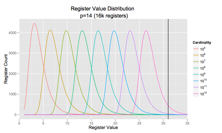
 E and n.)

A solution and a rebuttal

The natural move to start estimating cardinalities in the billions is to simply move to a larger hash space where the hash collision probability becomes negligibly small. This is fairly straightforward since most good hash functions give you at least 64-bits of entropy these days and it’s also the size of a machine word. There’s really no downside to moving to the larger hash space, from an engineering perspective. However, the Google researchers go one step further: they increase the register width by one bit (to 6), as well, ostensibly to be able to support the higher possible register values in the 64-bit setting. I contend this is unnecessary. If we look at the distribution of register values for a given cardinality, we see that it takes about a trillion elements before a 5-bit register overflows (at the black line):

regdistro-1

The distributions above come from the LogLog paper, on page 611, right before formula 2. Look for \mathbb{P}_{\nu}(M = k).

Consider the setting in the paper where p = \log_2(m) = 14. Let’s says we wanted to safely count into the 100 billion range. If we have L = p + (2^5 - 1) = 14 + 31 = 45 then our new “large range correction” boundary is roughly one trillion, per the adapted formula above. As you can see from the graph below, even at p = 10, L = 41 the large range correction only kicks in at a little under 100 billion!

lrcvsmrv-2

The black line is the cutoff for a 5-bit register, and the points are plotted when the total number of hash bits required reaches 40, 50, and 60.

The real question though is all this practically useful? I would argue no: there are no internet phenomena that I know of that are producing more than tens of billions of distinct values, and there’s not even a practical way of empirically testing the accuracy of HLL at cardinalities above 100 billion. (Assuming you could insert 50 million unique, random hashed values per second, it would take half an hour to fill an HLL to 100 billion elements, and then you’d have to repeat that 5000 times as they do in the paper for a grand total of 4 months of compute time per cardinality in the range.)

[UPDATE: After talking with Marc Nunkesser (one of the authors) it seems that Google may have a legitimate need for both the 100 billion to trillion range right now, and even more later, so I retract my statement! For the rest of us mere mortals, maybe this section will be useful for picking whether or not you need five or six bits.]

At AK we’ve run a few hundred test runs at 1, 1.5, and 2 billion distinct values under the p = 10-14, L = 41-45 
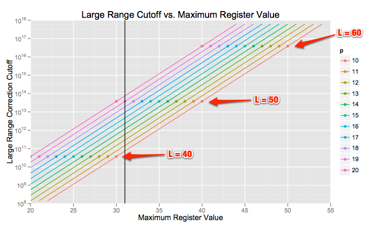
configuration range and found the relative error to be identical to that of lower cardinalities (in the millions of DVs). There’s really no reason to inflate the storage requirements for large cardinality HLLs by 20% simply because the hash space has expanded. Furthermore, you can do all kinds of simple tricks like storing an offset as metadata (which would only require at most 5 bits) for a whole HLL and storing the register values as the difference from that base offset, in order to make use of a larger hash space.

Small Cardinality Estimation

Simply put, the paper introduces a second small range correction between the existing one (linear counting) and the “normal” harmonic mean estimator (E in the original paper) in order to eliminate the “large” jump in relative error around the boundary between the two estimators.

They empirically calculate the bias of E and create a lookup table for various p, for 200 values less than 5 \cdot 2^p with a correction to the overestimate of E. They interpolate between the 200 reference points to determine the correction to apply for any given raw E value. Their plots give compelling evidence that this bias correction makes a difference in the m to 5m cardinality range (cuts 95th percentile relative error from about 2% to 1.2%).

I’ve been a bit terse about this improvement since sadly it doesn’t help us at AK much because most of our data is Zipfian. Few of our reporting keys live in the narrow cardinality range they are optimizing: they either wallow in the linear counting range or shoot straight up into the normal estimator range.

Nonetheless, if you find you’re doing a lot of DV counting in this range, these corrections are pretty cheap to implement (as they’ve provided numerical values for all the cutoffs and bias corrections in the appendix.)

Sparse representation

The general theme of this optimization isn’t particularly new (our friends at MetaMarkets mentioned it in this post): for smaller cardinality HLLs there’s no need to materialize all the registers. You can get away with just materializing the set registers in a map. The paper proposes a sorted map (by register index) with a hash map off the side to allow for fast insertions. Once the hash map reaches a certain size, its entries are batch-merged into the sorted list, and once the sorted list reaches the size of the materialized HLL, the whole thing is converted to the fully-materialized representation.

Aside: Though the hash map is a clever optimization, you could skip it if you didn’t want the added complexity. We’ve found that the simple sorted list version is extremely fast (hundreds of thousands of inserts per second). Also beware the variability of the the batched sort-and-merge cost every time the hash map repeatedly outgrows its limits and has to be merged into the sorted list. This can add significant latency spikes to a streaming system, whereas a one-by-one insertion sort to a sorted list will be slower but less variable.

The next bit is very clever: they increase p when the HLL is in the sparse representation because of the saved space. Since they’re already storing entries in 32-bit integers, they increase p to p^{\prime} = 31 - \mbox{regWidth} = 31 - 6 = 25. (I’ll get to the leftover bit in a second!) This gives them increased precision which they can simply “fold” down when converting from the sparse to fully materialized representation. Even more clever is their trick of not having to always store the full register value as the value of an entry in the map. Instead, if the longer register index encodes enough bits to determine the value, they use the leftover bit I mentioned before to signal as much.

HLL++ sparse encoding explanation

In the diagram, p and p^{\prime} are as in the Google paper, and q and q^{\prime} are the number of bits that need to be examined to determine \rho for either the p or p^{\prime} regime. I encourage you to read section 5.3.3 as well as EncodeHash and DecodeHash in Figure 8 to see the whole thing. [UPDATE: removed the typo section as it has been fixed in the most recent version of the paper (linked at the top)]

The paper also tacks on a difference encoding (which works very well because it’s a sorted list) and a variable length encoding to the sparse representation to further shrink the storage needed, so that the HLL can use the increased register count, p^{\prime}, for longer before reverting to the fully materialized representation at p. There’s not much to say about it because it seems to work very well, based on their plots, but I’ll note that in no way is that type of encoding suitable for streaming or “real-time” applications. The encode/decode overhead simply takes an already slow (relative to the fully materialized representation) sparse format and adds more CPU overhead.

Conclusion

The researchers at Google have done a great job with this paper, meaningfully tackling some hard engineering problems and showing some real cleverness. Most of the optimizations proposed work very well in a database context, where the HLLs are either being used as temporary aggregators or are being stored as read-only data, however some of the optimizations aren’t suitable for streaming/”real-time” work. On a more personal note, it’s very refreshing to see real algorithmic engineering work being published from industry. Rob, Matt, and I just got back from New Orleans and SODA / ALENEX / ANALCO and were hoping to see more work in this area, and Google sure did deliver!


Appendix

Sebastiano Vigna brought up the point that 6-bit registers are necessary for counting above 4 billion in the comments. I addressed it in the original post (see “A solution and a rebuttal“) but I’ll lay out the math in a bit more detail here to show that you can easily count above 4 billion with only 5-bit registers.

If you examine the original LogLog paper (the same as mentioned above) you’ll see that the register distribution for LogLog (and HyperLogLog consequently) registers is

\displaystyle \mathbb{P}_{\nu}(M > k) = 1 - \mathbb{P}_{\nu}(M \le k) = 1 - \Big(1 - \frac{1}{2^k}\Big)^{\nu}

where k is the register value and \nu is the number of (distinct) elements a register has seen.

So, I assert that 5 bits for a register (which allows the maximum value to be 31) is enough to count to ten billion without any special tricks. Let’s fix p=14 and say we insert 10^{10} distinct elements. That means, any given register will see about \frac{10^{10}}{2^p} = \frac{10^{10}}{2^{14}} = \approx 6.1 \times 10^5 elements assuming we have a decent hash function. So, the probability that a given register will have a value greater than 31 is (per the LogLog formula given above)

\displaystyle \mathbb{P}_{\nu}(M > 31) = 1 - \mathbb{P}_{\nu}(M \le 31) = 1 - \Big(1 - \frac{1}{2^{31}}\Big)^{6.1 \times 10^5} \approx 0.00028

and hence the expected number of registers that would overflow is approximately 2^{14} \times 0.00028 \approx 4.5. So five registers out of sixteen thousand would overflow. I am skeptical that this would meaningfully affect the cardinality computation. In fact, I ran a few tests to verify this and found that the average number of registers with values greater than 31 was 4.5 and the relative error had the same standard deviation as that predicted by the paper, 1.04/\sqrt{m}.

For argument, let’s assume that you find those five overflowed registers to be unacceptable. I argue that you could maintain an offset in 5 bits for the whole HLL that would allow you to still use 5 bit registers but exactly store the value of every register with extremely high probability. I claim that with overwhelmingly high probability, every register the HLL used above is greater than 15 and less than or equal to 40. Again, we can use the same distribution as above and we find that the probability of a given register being outside those bounds is

\mathbb{P}_{\nu}(M < 15) \approx 10^{-162} and

\mathbb{P}_{\nu}(M > 40) \approx 10^{-7}.

Effectively, there are no register values outside of [15,40]. Now I know that I can just store 15 in my offset and the true value minus the offset (which now fits in 5 bits) in the actual registers.