HLL talk at SFPUG

I had the pleasure of speaking at the SF PostgreSQL User Group’s meetup tonight about sketching, the history of HLL, and our implementation of HLL as a PG extension. My slides are embedded below and you can get a PDF copy here. Be sure to click the gear below to show speaker’s notes for context!

If video is made available, I’ll post an update with a link!

Open Source Release: java-hll

We’re happy to announce our newest open-source project, java-hll, a HyperLogLog implementation in Java that is storage-compatible with the previously released postgresql-hll and js-hll implementations. And as the rule of three dictates, we’ve also extracted the storage specification that makes them interoperable into it’s own repository. Currently, all three implementations support reading storage specification v1.0.0, while only the PostgreSQL and Java implementations fully support writing v1.0.0. We hope to bring the JS implementation up to speed, with respect to serialization, shortly.

Open Source Release: js-hll

One of the first things that we wanted to do with HyperLogLog when we first started playing with it was to support and expose it natively in the browser. The thought of allowing users to directly interact with these structures — perform arbitrary unions and intersections on effectively unbounded sets all on the client — was exhilarating to us. We knew it could be done but we simply didn’t have the time.

Fast forward a few years to today. We had finally enough in the meager science/research budget to pick up an intern for a few months and as a side project I tasked him with turning our dream into a reality. Without further ado, we are pleased to announce the open-source release of AK’s HyperLogLog implementation for JavaScript, js-hll. We are releasing this code under the Apache License, Version 2.0 matching our other open source offerings.

We knew that we couldn’t just release a bunch of JavaScript code without allowing you to see it in action — that would be a crime. We passed a few ideas around and the one that kept bubbling to the top was a way to kill two birds with one stone. We wanted something that would showcase what you can do with HLL in the browser and give us a tool for explaining HLLs. It is typical for us to explain how HLL intersections work using a Venn diagram. You draw some overlapping circles with a broder that represents the error and you talk about how if that border is close to or larger than the intersection then you can’t say much about the size of that intersection. This works just ok on a whiteboard but what you really want is to just build a visualization that allows you to select from some sets and see the overlap. Maybe even play with the precision a little bit to see how that changes the result. Well, we did just that!

Click above to interact with the visualization

Click above to interact with the visualization

Note: There’s more interesting math in the error bounds that we haven’t explored. Presenting error bounds on a measurement that cannot mathematically be less than zero is problematic. For instance, if you have a ruler that can only measure to 1/2″ and you measure an object that truly is 1/8″ long you can say “all I know is this object measures under 0.25 inches”. Your object cannot measure less than 0 inches, so you would never say 0 minus some error bound. That is, you DO NOT say 0.0 ± 0.25 inches.  Similarly with set intersections there is no meaning to a negative intersection. We did some digging and just threw our hands up and tossed in what we feel are best practices. In the js-hll code we a) never show negative values and b) we call “spurious” any calculation that results in an answer within 20% of the error bound. If you have a better answer, we would love to hear it!

Doubling the Size of an HLL Dynamically – Extra Bits…

Author’s Note: This post is related to a few previous posts on the HyperLogLog algorithm.  See Matt’s overview of the algorithm, and see this for an overview of “folding” or shrinking HLLs in order to perform set operations. It is also the final post in a series on doubling the number of bins in HLLs. The first post dealt with the recovery time after doubling, and the second dealt with doubling’s accuracy when taking unions of two HLLs.

Introduction

The main draw to the HyperLogLog algorithm is its ability to make accurate cardinality estimates using small, fixed memory.  In practice, there are two choices a user makes which determine how much memory the algorithm will use: the number of registers (bins) and the size of each register (how high they can count).  As Timon discussed previously, increasing the size of each register will only increase the accuracy if the true cardinality of the stream is HUGE.

Recall that HyperLogLog (and most other streaming algorithms) is designed to work with a fixed number of registers, m, which is chosen as a function of the expected cardinality to approximate. We track a great number of different cardinality streams and in this context it is useful for us to not have one fixed value of m, but to have this evolve with the needs of a given estimation.

We are thus confronted with many engineering problems, some of which we have already discussed. In particular, one problem is that the neat feature of sketches, namely that they allow for an estimate of the cardinality of the union of multiple streams at no cost, depends on having sketches of the same size.

We’ve discussed how to get around this by folding HLLs, though with some increase in error. We’ve also explored a few options on how to effectively perform a doubling procedure. However, we started to wonder if any improvements could be made by using just a small amount of extra memory, say an extra bit for each register. In this post we will discuss one such idea and its use in doubling. Note: we don’t talk about quadrupling or more. We limit ourselves to the situation where HLL sketches only differ in m‘s by 1.

The Setup

One of the downfalls in doubling is that it there is no way to know, after doubling, whether a value belongs in its bin or its partner bin. Recall that a “partner bin” is the register that could have been used had our “prefix” (the portion of the hashed value which is used to decide which register to update) been one bit longer. If the binary representation of the bin index used only two bits of the hashed value, e.g. 01, then in an HLL that used a three-bit index, the same hashed value could have been placed in the bin whose index is either 101 or 001. Since 001 and 01 are the same number, we call 101 the “partner bin”. (See the “Key Processing” section in Set Operations On HLLs of Different Sizes).

Consider an example where we have an HLL with 2^{10} bins.The k^{th} bin has the value 7 in it, and after doubling we guess that its partner bin, at index (2^{10} + k)^{th}, should have a 5 in it. It is equally likely that the k^{th} bin should have the 5 in it and the (2^{10}+k)^{th} bin should have the 7 in it (since the “missing” prefix bit could have been a 1 or a 0)! Certainly the arrangement doesn’t change the basic cardinality estimate, but once we start getting involved with unions, the arrangement can make a very large difference.

To see how drastic the consequences can be, let’s look at a simple example. Suppose we start with an HLL with 2 bins and get the value 6 in each of its bins. Then we run the doubling procedure and decide that the partner bins should both have 1’s in them. With this information, it is equally likely that both of the arrangements below, “A” and “B”, could be the “true” larger HLL.

arrangement

Further suppose we have some other data with which we wish to estimate the union. Below, I’ve diagrammed what happens when we take the union.

union_diag

Arrangement A leads to a cardinality estimate (of the union) of about 12 and Arrangement B leads to a cardinality estimate (of the union) of about 122. This is an order of magnitude different! Obviously not all cases are this bad, but this example is instructive. It tells us that knowing the true location of each value is very important. We’ve attempted to improve our doubling estimate by keeping an extra bit of information as we will describe below.

The Algorithm

Suppose we have an HLL with m bins. Let’s keep another array of data which holds m total bits, one for each bin — we will call these the “Cached Values.” For each bin, we keep a 0 if the value truly belongs in the bin in which it was placed (i.e. if, had we run an HLL with 2m bins, the value would have been placed in the first m bins in the HLL), and we keep a 1 if the value truly belongs in the partner bin of the one in which it was placed (i.e. if, had we run an HLL with 2m bins, the value would have been placed in the last m bins). See the image below for an example. Here we see two HLLs which have processed the same data. The one on the left is half the size and collects the cached values as it runs on the data. The one on the right is simply the usual HLL algorithm run on the same data.

swap_diag

Looking at the first row of the small HLL (with m bins), the 0 cache value means that the 2 “belongs” in the top half of the large HLL, i.e. if we had processed the stream using a larger HLL the 2 would be in the same register. Essentially this cached bit allows you to know exactly where the largest value in a bin was located in the larger HLL (if the i^{th} bin has value V and cached value S, we place the value V in the S * 2^{\log{m}} + i = (S\cdot m + i)^{th} bin).

Doubling Bit Diagram

In practice, when we double, we populate the doubled HLL first with the (now correct location) bin values from the original HLL then we fill the remaining bins by using our “Proportion Doubling” algorithm.

Before we begin looking at the algorithm’s performance, let’s think about how much extra space this requires. In our new algorithm, notice that for each bin, we keep around either a zero or a one as its cached value. Hence, we require only one extra bit per bin to accommodate the cached values. Our implementation of HLL requires 5 bits per bin, since we want to be able to include values up to 2^5 -1= 31 in our bins. Thus, a standard HLL with m bins, requires 5m bits. Hence, this algorithm requires 5m + m = 6m bits (with the extra m bins representing the cached values). This implies that this sketch requires 20% more space.

The Data

Recall in the last post in this series, we explored doubling with two main strategies: Random Estimate (RE) and Proportion Doubling (PD). We did the same here, though using the additional information from this cached bit. We want to know a few things:

  • Does doubling using a cache bit work? i.e. is it better to fold the bigger one or double the smaller one when comparing HLL’s of different sizes?
  • Does adding in a cache bit change which doubling strategy is preferred (RE or PD)?
  • Does the error in union estimate depend on intersection size as we have seen in the past?
Experimental Setup

Is it better to double or fold?

For each experiment we took 2 sets of data (each generated from 200k random keys) and estimated the intersection size between them using varying methods.

  • “Folded”: estimate by filling up an HLL with log_{2}(m) = 10 and  comparing it to a folded HLL starting from log_{2}(m) = 11 and folded down log_{2}(m) = 10
  • “Large”: estimate by using two HLL’s of a larger HLL of log_{2}(m) = 11.  This is effectively a lower bound for our doubling approaches.
  • “Doubled – PD”: estimate by taking an HLL of log_{2}(m) = 10 and double it up to log_{2}(m) = 11 using the Proportion Doubling strategy.  Once this larger HLL is approximated we estimate the intersection with another HLL of native size log_{2}(m) = 11
  • “Doubled – RE”: estimate by taking an HLL of log_{2}(m) = 10 and doubling up to log_{2}(m) = 11 using Random Estimate strategy.

We performed an experiment 300 times at varying intersection sizes from 0 up to 200k (100%) overlapping elements between sets (in steps of 10k). The plots below show our results (and extrapolate between points).

Doubling_bias

The graph of the mean error looks pretty bad for Random Estimate doubling. Again we see that the error depends heavily on the intersection size and becomes more biased as the set’s overlap more. On the other hand, Proportion Doubling was much more successful  (recall that this strategy forces the proportion of bins in the to-be-doubled HLL and the HLL with which we will union it to be equal before and after doubling.)  It’s possible there is some error bias with small intersections but we would need to run more trials to know for sure. As expected, the “Folded” and the “Large” are centered around zero. But what about the spread of the error?

Doubling_spread

The Proportion Doubling strategy looks great! In my last post on this subject, we found that this doubling strategy (without the cached part) really only worked well in the large intersection size regime, but here, with the extra cache bits, we seem to avoid that. Certainly the large intersection regime is where the standard deviation is lowest, but for every intersection size, it is significantly lower than that of the smaller HLL. This suggests that one of our largest sources of error when we use doubling in conjunction with unions is related to our lack of knowledge of the arrangement of the bins (i.e. when doubling, we do not know which of the two partner bins gets the larger, observed value). So it appears that the strategy of keeping cache bits around does indeed work, provided you use a decent doubling scheme.

Interestingly, it is always much better to double a smaller cache HLL than to fold a larger HLL when comparing sketches of different sizes. This is represented above by the lower error of the doubled HLL than the small HLL. The error bounds do seem to depend on the size of the intersection between the two sets but this will require more work to really understand how, especially in the case of Proportion Doubling.

Notes:  In this work we focus solely on doubling a HLL sketch and then immediately using this new structure to compute set operations. It would be interesting to see if set operation accuracy changes as a doubled HLL goes through its “recovery” period under varying doubling methods. It is our assumption that nothing out of the ordinary would come of this, but we definitely could be wrong. We will leave this as an exercise for the reader.

Summary

We’ve found an interesting way of trading space for accuracy with this cached bit method, but there are certainly other ways of using an extra bit or two (per bucket). For instance, we could keep more information about the distribution of each bin by keeping a bit indicating whether or not the bin’s value minus one has been seen. (If the value is k, keep track of whether k-1 has shown up.)

We should be able to use any extra piece of information about the distribution or position of the data to help us obtain a more accurate estimate. Certainly, there are a myriad of other ideas ways of storing a bit or two of extra information per bin in order to gain a little leverage — it’s just a matter of figuring out what works best. We’ll be messing around more with this in the coming weeks, so if you have any ideas of what would work best, let us know in the comments!

(P.S. A lot of our recent work has been inspired by Flajolet et al.’s paper on PCSA – check out our post on this here!)

Thanks to Jeremie Lumbroso for his kind input on this post. We are much indebted to him and hopefully you will see more from our collaboration.

Sketch of the Day: Probabilistic Counting with Stochastic Averaging (PCSA)

Before there was LogLog, SuperLogLog or HyperLogLog there was Probabilistic Counting with Stochastic Averaging (PCSA) from the seminal work “Probabilistic Counting Algorithms for Data Base Applications” (also known as the “FM Sketches” due to its two authors, Flajolet and Martin). The basis of PCSA matches that of the other Flajolet distinct value (DV) counters: hash values from a collection into binary strings, use patterns in those strings as indicators for the number of distinct values in that collection (bit-pattern observables), then use stochastic averaging to combine m trials into a better estimate. Our HyperLogLog post has more details on these estimators as well as stochastic averaging.

Observables

The choice of observable pattern in PCSA comes from the knowledge that in a collection of randomly generated binary strings, the following probabilities occur:

\begin{aligned}  &P( ..... 1) &= 2^{-1} \\  &P( .... 10) &= 2^{-2} \\  &P( ... 100) &= 2^{-3}  \end{aligned}

\vdots

P(...10^{k-1}) = 2^{-k}

For each value added to the DV counter, a suitable hash is created and the position of the least-significant (right-most) 1 is determined. The corresponding position in a bitmap is updated and stored. I’ve created the simulation below so that you can get a feel for how this plays out.

Bit Pattern Simulation

Click above to run the bit-pattern simulation

(All bit representations in this post are numbered from 0 (the least-significant bit) on the right. This is the opposite of the direction in which they’re represented in the paper.)

Run the simulation a few times and notice how the bitmap is filled in. In particular, notice that it doesn’t necessarily fill in from the right side to the left — there are gaps that exist for a time that eventually get filled in. As the cardinality increases there will be a block of 1s on the right (the high probability slots), a block of 0s on the left (the low probability slots) and a “fringe” (as Flajolet et al. called it) of 1s and 0s in the middle.

I added a small pointer below the bitmap in the simulation to show how the cardinality corresponds to the expected bit position (based on the above probabilities). Notice what Flajolet et al. saw when they ran this same experiment: the least-significant (right-most) 0 is a pretty good estimator for the cardinality! In fact when you run multiple trials you see that this least-significant 0 for a given cardinality has a narrow distribution. When you combine the results with stochastic averaging it leads to a small relative error of 0.78 / \sqrt{m} and estimates the cardinality of the set quite well. You might have also observed that the most-significant (left-most) 1 can also be used for an estimator for the cardinality but it isn’t as clear-cut. This value is exactly the observable used in LogLog, SuperLogLog and HyperLogLog and does in fact lead to the larger relative error of 1.04 / \sqrt{m} (in the case of HLL).

Algorithm

The PCSA algorithm is elegant in its simplicity:

m = 2^b # with b in [4...16]

bitmaps = [[0]*32]*m # initialize m 32bit wide bitmaps to 0s

##############################################################################################
# Construct the PCSA bitmaps
for h in hashed(data):
    bitmap_index = 1 + get_bitmap_index( h,b ) # binary address of the rightmost b bits
    run_length = run_of_zeros( h,b ) # length of the run of zeroes starting at bit b+1
    bitmaps[ bitmap_index ][ run_length ] = 1 # set the bitmap bit based on the run length observed

##############################################################################################
# Determine the cardinality
phi = 0.77351
DV = m / phi * 2 ^ (sum( least_sig_bit( bitmap ) ) / m) # the DV estimate

Stochastic averaging is accomplished via the arithmetic mean.

You can see PCSA in action by clicking on the image below.

HyperLogLog Simulation

Click above to run the PCSA simulation

There is one point to note about PCSA and small cardinalities: Flajolet et al. mention that there are “initial nonlinearities” in the algorithm which result in poor estimation at small cardinalities (n/m \approx 10 \, \text{to} \, 20 ) which can be dealt with by introducing corrections but they leave it as an exercise for the reader to determine what those corrections are. Scheuermann et al. did the leg work in “Near-Optimal Compression of Probabilistic Counting Sketches for Networking Applications” and came up with a small correction term (see equation 6). Another approach is to simply use the linear (ball-bin) counting introduced in the HLL paper.

Set Operations

Just like HLL and KMV, unions are trivial to compute and lossless. The PCSA sketch is essentially a “marker” for runs of zeroes, so to perform a union you merely bit-wise OR the two sets of bitmaps together. Folding a PCSA down to a smaller m works the same way as HLL but instead of HLL’s max you bit-wise OR the bitmaps together. Unfortunately for intersections you have the same issue as HLL, you must perform them using the inclusion/exclusion principle. We haven’t done the plots on intersection errors for PCSA but you can imagine they are similar to HLL (and have the benefit of the better relative error 0.78 / \sqrt{m}).

PCSA vs. HLL

That fact that PCSA has a better relative error than HyperLogLog with the same number of registers (1.04 / 0.78 \approx 1.33 ) is slightly deceiving in that m (the number of stored observations) are different sizes. A better way to look at it is to fix the accuracy of the sketches and see how they compare. If we would like to have the same relative error from both sketches we can see that the relationship between registers is:

\text{PCSA}_{RE} = \text{HLL}_{RE}

\dfrac{0.78}{\sqrt{m_{\scriptscriptstyle PCSA}}} = \dfrac{1.04}{\sqrt{m_{\scriptscriptstyle HLL}}}

m_{\scriptscriptstyle PCSA} = \left( \dfrac{0.78}{1.04} \right)^2 m_{\scriptscriptstyle HLL} \approx 0.563 \ m_{\scriptscriptstyle HLL}

Interestingly, PCSA only needs a little more than half the registers of an HLL to reach the same relative error. But this is also deceiving. What we should be asking is what is the size of each sketch if they provide the same relative error? HLL commonly uses a register width of 5 bits to count to billions whereas PCSA requires 32 bits. That means a PCSA sketch with the same accuracy as an HLL would be:

\begin{aligned}  \text{Size of PCSA} &= 32 \text{bits} \ m_{\scriptscriptstyle PCSA} = 32 \text{bits} \, ( 0.563 \ m_{\scriptscriptstyle HLL} )   \\  \\  \text{Size of HLL} &= 5 \text{bits} \ m_{\scriptscriptstyle HLL}  \end{aligned}

Therefore,

\dfrac{\text{Size of PCSA}} {\text{Size of HLL}} = \dfrac{32 \text{bits} \, ( 0.563 \ m_{\scriptscriptstyle HLL} )}{5 \text{bits} \ m_{\scriptscriptstyle HLL}} \approx 3.6

A PCSA sketch with the same accuracy is 3.6 times larger than HLL!

Optimizations

But what if you could make PCSA smaller by reducing the size of the bitmaps? Near the end of the paper in the Scrolling section, Flajolet et al. bring up the point that you can make the bitmaps take up less space. From the simulation you can observe that with a high probability there is a block of consecutive 1s on the right side of the bitmap and a block of consecutive 0s on the left side of the bitmap with a fringe in between. If one found the “global fringe” — that is the region defined by the left-most 1 and right-most 0 across all bitmaps — then only those bits need to be stored (along with an offset value). The authors theorized that a fringe width of 8 bits would be sufficient (though they fail to mention if there are any dependencies on the number of distinct values counted). We put this to the test.

PCSA with Fringe Cardinality Error

For a plot with larger m values, click here.

In our simulations it appears that a fringe width of 12 bits is necessary to provide an unbiased estimator comparable to full-fringe PCSA (32-bit) for the range of distinct values we analyzed. (Notice the consistent bias of smaller fringe sizes.) There are many interesting reasons that this “fringe” concept can fail. Look at the notes to this post for more. If we take the above math and update 32 to 12 bits per register (and include the 32 bit offset value) we get:

\begin{aligned}  \dfrac{\text{Size of PCSA}} {\text{Size of HLL}}  &= \dfrac{12 \text{bits} \, ( 0.563 \ m_{\scriptscriptstyle HLL} ) + 32\text{bits}} {5 \text{bits} \cdot m_{\scriptscriptstyle HLL}}  \\  \\  &= \dfrac{12 \text{bits} \, ( 0.563 \ m_{\scriptscriptstyle HLL} )} {5 \text{bits} \cdot m_{\scriptscriptstyle HLL}} + \dfrac{32\text{bits}} {5 \text{bits} \cdot m_{\scriptscriptstyle HLL}}  \\  \\  &\approx 1.35 \text{ (for }m\gg64 \text{)}    \end{aligned}

This is getting much closer to HLL! The combination of tighter bounds on the estimate and the fact that the fringe isn’t really that wide in practice result in PCSA being very close to the size of the much lauded HLL. This got us thinking about further compression techniques for PCSA. After all, we only need to get the sketch about 1/3 smaller to be comparable in size to HLL. In a future post we will talk about what happens if you Huffman code the PCSA bitmaps and the tradeoffs you make when you do this.

Summary

PCSA provides for all of the goodness of HLL: very fast updates making it suitable for real-time use, small footprint compared to the information that it provides, tunable accuracy and unions. The fact that it has a much better relative error per register than HLL indicates that it should get more credit than it does. Unfortunately, each bitmap in PCSA requires more space than HLL and you still get less accuracy per bit. Look for a future post on how it is possible to use compression (e.g. Huffman encoding) to reduce the number of bits per bitmap, thus reducing the error per bit to match that of HLL, resulting in an approach that matches HLL in size but exceeds its precision!

Notes on the Fringe

While we were putting this post together we discovered many interesting things to look at with respect to fringe optimization. One of the questions we wanted to answer was “How often does the limited size of the fringe muck up a bitmap?” Below is a plot that shows how often any given sketch had a truncation event (that affected the DV estimate) in the fringe of any one of its bitmaps for a given fringe width (i.e. some value could not be stored in the space available).

Truncated_Observations-2

Note that this is an upper bound on the error that could be generated by truncation. If you compare the number of runs that had a truncation event (almost all of the runs) with the error plot in the post it is quite shocking that the errors are as small as they are.

Since we might not get around to all of the interesting research here, we are calling out to the community to help! Some ideas:

  1. There are likely a few ways to improve the fringe truncation. Since PCSA is so sensitive to the least-significant 1 in each bitmap, it would be very interesting to see how different approaches affect the algorithm. For example, in our algorithm we “left” truncated meaning that all bitmaps had to have a one in the least-significant position of the bitmap in order to move up the offset. It would be interesting to look at “right” truncation. If one bitmap is causing many of the others to not record incoming values perhaps it should be bumped up. Is there some math to back up this intuition?
  2. It is interesting to us that the fringe width truncation events are DV dependent. We struggled with the math on this for a bit before we just stopped. Essentially we want to know what is the width of the theoretical fringe? It obviously appears to be DV dependent and some sort of coupon collector problem with unequal probabilities. Someone with better math skills than us needs to help here.

Closing thoughts

We uncovered PCSA again as a way to go back to first principles and see if there are lessons to be learned that could be applied to HLL to make it even better. For instance, can all of this work on the fringe be applied to HLL to reduce the number of bits per register while still maintaining the same precision? HLL effectively records the “strandline” (what we call the left-most 1s). More research into how this strandline behaves and if it is possible to improve the storage of it through truncation could reduce the standard HLL register width from 5 bits to 4, a huge savings! Obviously, we uncovered a lot of open questions with this research and we feel there are algorithmic improvements to HLL right around the corner. We have done some preliminary tests and the results so far are intriguing. Stay tuned!

HyperLogLog Engineering: Choosing The Right Bits

Author’s Note: this is just a quick post about an engineering hiccup we ran into while implementing HyperLogLog features that aren’t mentioned in the original paper. We have an introduction to the algorithm and several other posts on the topic if you’re interested.

Say you had two HyperLogLog data structures with 5-bit-wide registers, one with log_{2}m = 11 and the other with log_{2}m = 15, and wanted to compute their union. You could just follow my colleague Chris’ advice and “fold” the larger one down to the size of the smaller one and then proceed as usual taking the pairwise max of the registers. This turns out to be a more involved process than Chris makes it out to be if you designed your HLL implementation in a particular way. For instance, if you use the 15 least(/most) significant bits of the 64-bit hashed input to determine register index and the next 30 bits to determine the register value, you end up in a tricky situation when you truncate the last 4 bits of the index to get the new 11-bit index.

bit string bad

If you imagine feeding the same element into an HLL of the smaller size, then the 4 bits you truncated from the index would have actually been used in the computation of the register value.

bit string bad after fold

You couldn’t simply take the original register value you computed, you’d have to take into account the new prefix added to the register value bit string. If the prefix has a 1 in it, you would recompute the run of zeroes on just the prefix (because you know it contains a 1 and thus all the information you need), and if not, you’d add the length of the prefix to the original register value computed. Not a ton of work, but having clutter like this in algorithmic code distracts the reader from the true intention. So how do we avoid this?

Well, you could say that it’s very, very unlikely that you’ll ever need more than 30 bits for your register value, so you could assume that the register width would remain constant forever and use the bottom 30 bits for your register value and the next log_{2}m bits for your register index. That way you could just truncate the last 4 bits of the index and know that your register value would still be the same. On the other hand, if you’re Google, that may not be true. In that case, what you should do is use the log_{2}m least (/most) significant bits of your hashed value for the register index and the 30 most (/least) significant bits for the register value.

bit string

Now you can just truncate the register index and use the original register value.

bit string after fold

If you’re using a good hash function like MurmurHash3 that gives you 128 bits of entropy, you could simply compute the register index from the first 64-bit word in the hash and compute the register value from the second 64-bit word and completely ignore this problem up to a mind-bending log_{2}m = 64 and register width of 6 (aka the heat death of the universe).

I know it’s not always possible to anticipate this problem in the early stages of implementing and vetting an algorithm, but hopefully with a bit of research the next time someone looks to implement HLL they’ll see this and learn from our mistake.

Doubling the Size of an HLL Dynamically – Unions

Author’s Note: This post is related to a few previous posts dealing with the HyperLogLog algorithm.  See Matt’s overview of the algorithm, and see this post for an overview of “folding” or shrinking HLLs in order to perform set operations. It is also the second in a series of three posts on doubling the number of bins of HLLs. The first post dealt with the recovery time after doubling and the next post will deal with ways to utilize an extra bit or two per bin.

Overview

Let’s say we have two streams of data which we’re monitoring with the HLL algorithm, and we’d like to get an estimate on the cardinality of these two streams combined, i.e. thought of as one large stream.  In this case, we have to take advantage of the algorithm’s built-in “unionfeature.  Done naively, the accuracy of the estimate will depend entirely on the the number of bins, m, of the smaller of the two HLLs.  In this case, to make our estimate more accurate, we would need to increase this m of one (or both) of our HLLs.  This post will investigate the feasibility of doing this; we will apply our idea of “doubling” to see if we can gain any accuracy.  We will not focus on intersections, since the only support the HyperLogLog algorithm has for intersections is via the inclusion/exclusion principle. Hence the error can be kind of funky for this – for a better overview of this, check out Timon’s post here. For this reason, we only focus on how the union works with doubling.

The Strategy: A Quick Reminder

In my last post we discussed the benefits and drawbacks of many different doubling strategies in the context of recovery time of the HLL after doubling. Eventually we saw that two of our doubling strategies worked significantly better than the others. In this post, instead of testing many different strategies, we’ll focus instead on one strategy, “proportion doubling” (PD), and how to manipulate it to work best in the context of unions. The idea behind PD is to guess the approximate intersection cardinality of the two datasets and to force that estimate to remain after doubling. To be more specific, suppose we have an HLL A and an HLL B withn bins and 2n bins, respectively. Then we check what proportion of bins in A, call it p, agree with the bins in B. When we doubled A, we fill in the bins by randomly selecting p\cdot n bins, and filling them in with the value in the corresponding bins in B. To fill in the rest of the bins, we fill them in randomly according to the distribution.

The Naive Approach

To get some idea of how well this would work, I put the most naive strategy to the test. The idea was to run 100 trials where I took two HLLs (one of size 2^5 = 32 and one of size 2^6 = 64), ran 200K keys through them, doubled the smaller one (according to Random Estimate), and took a union. I had a hunch that the accuracy of our estimate after doubling would depend on how large the true intersection cardinality of the two datasets would be, so I ran this experiment for overlaps of size 0, 10K, 20K, etc. The graphs below are organized by the true intersection cardinality, and each graph shows the boxplot of the error for the trials.

pd_graphs_naiveThis graph is a little overwhelming and a bit of a strange way to display the data, but is useful for getting a feel for how the three estimates work in the different regimes.  The graph below is from the same data and just compares the “Small” and “Doubled” HLLs.  The shaded region represents the middle 50% of the data, and the blue dots represent the data points.

smoothed_naive_union_error

The first thing to notice about these graphs is the accuracy of the estimate in the small intersection regime. However, outside of this, the estimates are not very accurate – it is clearly a better choice to just use the estimate from the smaller HLL.

Let’s try a second approach. Above we noticed that the algorithm’s accuracy depended on the cardinality of the intersection. Let’s try to take that into consideration. Let’s use the “Proportion Doubling” (PD) strategy we discussed in our first post. That post goes more in depth into the algorithm, but the take away is that this doubling strategy preserves the proportion of bins in the two HLLs which agree. I ran some trials like I did above to get some data on this. The graphs below represent this.

pd_graphsHere we again, show the data in a second graph comparing just the “Doubled” and “Small” HLL estimates.  Notice how much tighter the middle 50% region is on the top graph (for the “Doubled” HLL).  Hence in the large intersection regime, we get very accurate estimates.

smoothed_pd_union_error

One thing to notice about the second set of graphs is how narrow the error bars are.  Even when the estimate is biased, it still has much smaller error.  Also, notice that this works well in the large intersection regime but horribly in the small intersection regime.  This suggests that we may be able to interpolate our strategies. The next set of graphs is for an attempt at this. The algorithm gets an estimate of the intersection cardinality, then decides to either double using PD, double using RE, or not double depending on whether the intersection is large, small, or medium.

hybridpic1

smoothed_hybrid_union_error

Here, the algorithm works well in the large intersection regime and doesn’t totally crap out outside of this regime (like the second algorithm), but doesn’t sustain the accuracy of the first algorithm in the small intersection regime. This is most likely because the algorithm cannot “know” which regime it is in and thus, must make a guess.  Eventually, it will guess wrong will severely underestimate the union cardinality. This will introduce a lot of error, and hence, our boxplot looks silly in this regime. The graph below shows the inefficacy of this new strategy. Notice that there are virtually no gains in accuracy in the top graph.

Conclusion

With some trickery, it is indeed possible to gain some some accuracy when estimating the cardinality of the union of two HLLs by doubling one.  However, in order for this to be feasible, we need to apply the correct algorithm in the correct regime. This isn’t a major disappointment since for many practical cases, it would be easy to guess which regime the HLLs should fall under and we could build in the necessary safeguards if we guess incorrectly.  In any case, our gains were modest but certainly encouraging!

Open Source Release: postgresql-hll

We’re happy to announce the first open-source release of AK’s PostgreSQL extension for building and manipulating HyperLogLog data structures in SQL, postgresql-hll. We are releasing this code under the Apache License, Version 2.0 which we feel is an excellent balance between permissive usage and liability limitation.

What is it and what can I do with it?

The extension introduces a new data type, hll, which represents a probabilistic distinct value counter that is a hybrid between a HyperLogLog data structure (for large cardinalities) and a simple set (for small cardinalities). These structures support the basic HLL methods: insert, union, and cardinality, and we’ve also provided aggregate and debugging functions that make using and understanding these things a breeze. We’ve also included a way to do schema versioning of the binary representations of hlls, which should allow a clear path to upgrading the algorithm, as new engineering insights come up.

A quick overview of what’s included in the release:

  • C-based extension that provides the hll data structure and algorithms
  • Austin Appleby’s MurmurHash3 implementation and SQL-land wrappers for integer numerics, bytes, and text
  • Full storage specification in STORAGE.markdown
  • Full function reference in REFERENCE.markdown
  • .spec file for rpmbuild
  • Full test suite

A quick note on why we included MurmurHash3 in the extension: we’ve done a good bit of research on the importance of a good hash function when using sketching algorithms like HyperLogLog and we came to the conclusion that it wouldn’t be very user-friendly to force the user to figure out how to get a good hash function into SQL-land. Sure, there are plenty of cryptographic hash functions available, but those are (computationally) overkill for what is needed. We did the research and found MurmurHash3 to be an excellent non-cryptographic hash function in both theory and practice. We’ve been using it in production for a while now with excellent results. As mentioned in the README, it’s of crucial importance to reliably hash the inputs to hlls.

Why did you build it?

The short answer is to power these two UIs:

On the left is a simple plot of the number of unique users seen per day and the number of cumulative unique users seen over the days in the month. The SQL behind this is very very straightforward:

SELECT report_date,
       #users as by_day,
       #hll_union_agg(users) as cumulative_by_day OVER (ORDER BY report_date ASC)
FROM daily_uniques
WHERE report_date BETWEEN '2013-01-01' AND '2013-01-31'
ORDER BY report_date ASC;

where daily_uniques is basically:

   Column    | Type | Modifiers 
-------------+------+-----------
 report_date | date | 
 users       | hll  |

Briefly, # is the cardinality operator which is operating on the hll result of the hll_union_agg aggregate function which unions the previous days’ hlls.

On the right is a heatmap of the percentage of an inventory provider’s users that overlap with another inventory provider. Essentially, we’re doing interactive set-intersection of operands with millions or billions of entries in milliseconds. This is intersection computed using the inclusion-exclusion principle as applied to hlls:

SELECT ip1.id as provider1,
       ip2.id as provider2,
       (#ip1.users + #ip2.users - #hll_union(ip1.users, ip2.users))/#ip1.users as overlap
FROM inventory_provider_stats ip1, inventory_provider_stats ip2
WHERE ip1.id <> ip2.id;

where inventory_provider_stats is basically:

   Column    | Type | Modifiers 
-------------+------+-----------
 id          | date | 
 users       | hll  |

(Some of you may note that the diagonal is labeled “exclusive reach” and is not represented in the query’s result set. That’s because the SQL above is a simplification of what’s happening. There’s some extra work done that replaces that the useless diagonal entries with the percent of the inventory provider’s users that are only seen on that inventory provider.)

We’ve been running this type of code in production for over a year now and are extremely pleased with its performance, ease of use, and expressiveness. Everyone from engineers to researchers to ops people to analysts have been using hlls in their daily reports and queries. We’re seeing product innovation coming from all different directions in the organization as a direct result of having these powerful data structures in an easily accessed and queried format. Dynamic COUNT(DISTINCT ...) queries that would have taken minutes or hours to compute from a fact table or would have been impossible in traditional cube aggregates return in milliseconds. Combine that speed with PostgreSQL’s window and aggregate functions and you have the ability to present interactive, rich distinct-value reporting over huge data sets. I’ll point you to the README and our blog posts on HyperLogLog for more technical details on storage, accuracy, and in-depth use cases.

I believe that this pattern of in-database probabilistic sketching is the future of interactive analytics. As our VP of Engineering Steve Linde said to me, “I can’t emphasize enough how much business value [sketches] deliver day in and day out.”

Our Commitment

Obviously we’re open-sourcing this for both philanthropic and selfish reasons: we’d love for more people to use this technology so that they can tell us all the neat uses for it that we haven’t thought of yet. In exchange for their insight, we’re promising to stay active in terms of stewardship and contribution of our own improvements. Our primary tool for this will be the GitHub Issues/Pull Request mechanism. We’d considered a mailing list but that seems like overkill right now. If people love postgresql-hll, we’ll figure something out as needed.

Please feel free to get in touch with us about the code on GitHub and about the project in general in the comments here. We hope to release additional tools that allow seamless Java application integration with the raw hll data in the future, so stay tuned!


Update

Looks Dimitri Fontaine wrote up a basic “how-to” post on using postgresql-hll here and another on unions here. (Thanks, Dimitri!) He brings up the issue that hll_add_agg() returns NULL when aggregating over an empty set when it should probably return an empty hll. Hopefully we’ll have a fix for that soon. You can follow the progress of the issue here.

HyperLogLog++: Google’s Take On Engineering HLL

Matt Abrams recently pointed me to Google’s excellent paper “HyperLogLog in Practice: Algorithmic Engineering of a State of The Art Cardinality Estimation Algorithm” [UPDATE: changed the link to the paper version without typos] and I thought I’d share my take on it and explain a few points that I had trouble getting through the first time. The paper offers a few interesting improvements that are worth noting:

  1. Move to a 64-bit hash function
  2. A new small-cardinality estimation regime
  3. A sparse representation

I’ll take a look at these one at a time and share our experience with similar optimizations we’ve developed for a streaming (low latency, high throughput) environment.

32-bit vs. 64-bit hash function

I’ll motivate the move to a 64-bit hash function in the context of the original paper a bit more since the Google paper doesn’t really cover it except to note that they wanted to count billions of distinct values.

Some math

In the original HLL paper, a 32-bit hash function is required with the caveat that measuring cardinalities in the hundreds of millions or billions would become problematic because of hash collisions. Specifically, Flajolet et al. propose a “large range correction” for when the estimate E is greater than 2^{32}/30.  In this regime, they replace the usual HLL estimate by the estimate

\displaystyle E^* := -2^{32} \mbox{log}\Big(1 - \frac{E}{2^{32}}\Big).

This reduces to a simple probabilistic argument that can be modeled with balls being dropped into bins. Say we have an L-bit hash. Each distinct value is a ball and each bin is designated by a value in the hash space.  Hence, you “randomly” drop a ball into a bin if the hashed value of the ball corresponds to the hash value attached to the bin.  Then, if we get an estimate E for the cardinality, that means that (approximately) E of our bins have values in them, and so there are 2^L - E empty bins.  The number of empty bins should be about 2^L e^{ - n/2^{L} }, where n is the number of balls.  Hence 2^{L} - E = 2^{L} e^{-n/2^{L}}.  Solving this gives us the formula he recommends using: -2^L \log(1 - \frac{E}{2^{L}}).

Aside:  The empty bins expected value comes from the fact that

E(\# \text{ of empty bins}) = m(1 - \frac{1}{m})^{n},

where m is the number of bins and n the number of balls.  This is pretty quick to show by induction.  Hence,

\displaystyle E(\#\text{ of empty bins}) \sim m e^{-n/m} as n \rightarrow \infty.

Again, the general idea is that the E ends up being some number smaller than n because some of the balls are getting hashed to the same value.  The correction essentially doesn’t do anything in the case when E is small compared to 2^L as you can see here. (Plotted is -\log(1 - x), where x represents E / 2^L, against the line y = x. The difference between the two graphs represents the difference between
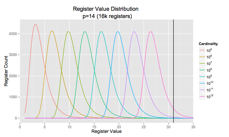
 E and n.)

A solution and a rebuttal

The natural move to start estimating cardinalities in the billions is to simply move to a larger hash space where the hash collision probability becomes negligibly small. This is fairly straightforward since most good hash functions give you at least 64-bits of entropy these days and it’s also the size of a machine word. There’s really no downside to moving to the larger hash space, from an engineering perspective. However, the Google researchers go one step further: they increase the register width by one bit (to 6), as well, ostensibly to be able to support the higher possible register values in the 64-bit setting. I contend this is unnecessary. If we look at the distribution of register values for a given cardinality, we see that it takes about a trillion elements before a 5-bit register overflows (at the black line):

regdistro-1

The distributions above come from the LogLog paper, on page 611, right before formula 2. Look for \mathbb{P}_{\nu}(M = k).

Consider the setting in the paper where p = \log_2(m) = 14. Let’s says we wanted to safely count into the 100 billion range. If we have L = p + (2^5 - 1) = 14 + 31 = 45 then our new “large range correction” boundary is roughly one trillion, per the adapted formula above. As you can see from the graph below, even at p = 10, L = 41 the large range correction only kicks in at a little under 100 billion!

lrcvsmrv-2

The black line is the cutoff for a 5-bit register, and the points are plotted when the total number of hash bits required reaches 40, 50, and 60.

The real question though is all this practically useful? I would argue no: there are no internet phenomena that I know of that are producing more than tens of billions of distinct values, and there’s not even a practical way of empirically testing the accuracy of HLL at cardinalities above 100 billion. (Assuming you could insert 50 million unique, random hashed values per second, it would take half an hour to fill an HLL to 100 billion elements, and then you’d have to repeat that 5000 times as they do in the paper for a grand total of 4 months of compute time per cardinality in the range.)

[UPDATE: After talking with Marc Nunkesser (one of the authors) it seems that Google may have a legitimate need for both the 100 billion to trillion range right now, and even more later, so I retract my statement! For the rest of us mere mortals, maybe this section will be useful for picking whether or not you need five or six bits.]

At AK we’ve run a few hundred test runs at 1, 1.5, and 2 billion distinct values under the p = 10-14, L = 41-45 
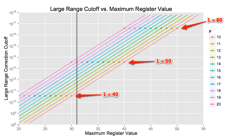
configuration range and found the relative error to be identical to that of lower cardinalities (in the millions of DVs). There’s really no reason to inflate the storage requirements for large cardinality HLLs by 20% simply because the hash space has expanded. Furthermore, you can do all kinds of simple tricks like storing an offset as metadata (which would only require at most 5 bits) for a whole HLL and storing the register values as the difference from that base offset, in order to make use of a larger hash space.

Small Cardinality Estimation

Simply put, the paper introduces a second small range correction between the existing one (linear counting) and the “normal” harmonic mean estimator (E in the original paper) in order to eliminate the “large” jump in relative error around the boundary between the two estimators.

They empirically calculate the bias of E and create a lookup table for various p, for 200 values less than 5 \cdot 2^p with a correction to the overestimate of E. They interpolate between the 200 reference points to determine the correction to apply for any given raw E value. Their plots give compelling evidence that this bias correction makes a difference in the m to 5m cardinality range (cuts 95th percentile relative error from about 2% to 1.2%).

I’ve been a bit terse about this improvement since sadly it doesn’t help us at AK much because most of our data is Zipfian. Few of our reporting keys live in the narrow cardinality range they are optimizing: they either wallow in the linear counting range or shoot straight up into the normal estimator range.

Nonetheless, if you find you’re doing a lot of DV counting in this range, these corrections are pretty cheap to implement (as they’ve provided numerical values for all the cutoffs and bias corrections in the appendix.)

Sparse representation

The general theme of this optimization isn’t particularly new (our friends at MetaMarkets mentioned it in this post): for smaller cardinality HLLs there’s no need to materialize all the registers. You can get away with just materializing the set registers in a map. The paper proposes a sorted map (by register index) with a hash map off the side to allow for fast insertions. Once the hash map reaches a certain size, its entries are batch-merged into the sorted list, and once the sorted list reaches the size of the materialized HLL, the whole thing is converted to the fully-materialized representation.

Aside: Though the hash map is a clever optimization, you could skip it if you didn’t want the added complexity. We’ve found that the simple sorted list version is extremely fast (hundreds of thousands of inserts per second). Also beware the variability of the the batched sort-and-merge cost every time the hash map repeatedly outgrows its limits and has to be merged into the sorted list. This can add significant latency spikes to a streaming system, whereas a one-by-one insertion sort to a sorted list will be slower but less variable.

The next bit is very clever: they increase p when the HLL is in the sparse representation because of the saved space. Since they’re already storing entries in 32-bit integers, they increase p to p^{\prime} = 31 - \mbox{regWidth} = 31 - 6 = 25. (I’ll get to the leftover bit in a second!) This gives them increased precision which they can simply “fold” down when converting from the sparse to fully materialized representation. Even more clever is their trick of not having to always store the full register value as the value of an entry in the map. Instead, if the longer register index encodes enough bits to determine the value, they use the leftover bit I mentioned before to signal as much.

HLL++ sparse encoding explanation

In the diagram, p and p^{\prime} are as in the Google paper, and q and q^{\prime} are the number of bits that need to be examined to determine \rho for either the p or p^{\prime} regime. I encourage you to read section 5.3.3 as well as EncodeHash and DecodeHash in Figure 8 to see the whole thing. [UPDATE: removed the typo section as it has been fixed in the most recent version of the paper (linked at the top)]

The paper also tacks on a difference encoding (which works very well because it’s a sorted list) and a variable length encoding to the sparse representation to further shrink the storage needed, so that the HLL can use the increased register count, p^{\prime}, for longer before reverting to the fully materialized representation at p. There’s not much to say about it because it seems to work very well, based on their plots, but I’ll note that in no way is that type of encoding suitable for streaming or “real-time” applications. The encode/decode overhead simply takes an already slow (relative to the fully materialized representation) sparse format and adds more CPU overhead.

Conclusion

The researchers at Google have done a great job with this paper, meaningfully tackling some hard engineering problems and showing some real cleverness. Most of the optimizations proposed work very well in a database context, where the HLLs are either being used as temporary aggregators or are being stored as read-only data, however some of the optimizations aren’t suitable for streaming/”real-time” work. On a more personal note, it’s very refreshing to see real algorithmic engineering work being published from industry. Rob, Matt, and I just got back from New Orleans and SODA / ALENEX / ANALCO and were hoping to see more work in this area, and Google sure did deliver!


Appendix

Sebastiano Vigna brought up the point that 6-bit registers are necessary for counting above 4 billion in the comments. I addressed it in the original post (see “A solution and a rebuttal“) but I’ll lay out the math in a bit more detail here to show that you can easily count above 4 billion with only 5-bit registers.

If you examine the original LogLog paper (the same as mentioned above) you’ll see that the register distribution for LogLog (and HyperLogLog consequently) registers is

\displaystyle \mathbb{P}_{\nu}(M > k) = 1 - \mathbb{P}_{\nu}(M \le k) = 1 - \Big(1 - \frac{1}{2^k}\Big)^{\nu}

where k is the register value and \nu is the number of (distinct) elements a register has seen.

So, I assert that 5 bits for a register (which allows the maximum value to be 31) is enough to count to ten billion without any special tricks. Let’s fix p=14 and say we insert 10^{10} distinct elements. That means, any given register will see about \frac{10^{10}}{2^p} = \frac{10^{10}}{2^{14}} = \approx 6.1 \times 10^5 elements assuming we have a decent hash function. So, the probability that a given register will have a value greater than 31 is (per the LogLog formula given above)

\displaystyle \mathbb{P}_{\nu}(M > 31) = 1 - \mathbb{P}_{\nu}(M \le 31) = 1 - \Big(1 - \frac{1}{2^{31}}\Big)^{6.1 \times 10^5} \approx 0.00028

and hence the expected number of registers that would overflow is approximately 2^{14} \times 0.00028 \approx 4.5. So five registers out of sixteen thousand would overflow. I am skeptical that this would meaningfully affect the cardinality computation. In fact, I ran a few tests to verify this and found that the average number of registers with values greater than 31 was 4.5 and the relative error had the same standard deviation as that predicted by the paper, 1.04/\sqrt{m}.

For argument, let’s assume that you find those five overflowed registers to be unacceptable. I argue that you could maintain an offset in 5 bits for the whole HLL that would allow you to still use 5 bit registers but exactly store the value of every register with extremely high probability. I claim that with overwhelmingly high probability, every register the HLL used above is greater than 15 and less than or equal to 40. Again, we can use the same distribution as above and we find that the probability of a given register being outside those bounds is

\mathbb{P}_{\nu}(M < 15) \approx 10^{-162} and

\mathbb{P}_{\nu}(M > 40) \approx 10^{-7}.

Effectively, there are no register values outside of [15,40]. Now I know that I can just store 15 in my offset and the true value minus the offset (which now fits in 5 bits) in the actual registers.

HLL Intersections

Why?

The intersection of two streams (of user ids) is a particularly important business need in the advertising industry. For instance, if you want to reach suburban moms but the cost of targeting those women on a particular inventory provider is too high, you might want to know about a cheaper inventory provider whose audience overlaps with the first provider. You may also want to know how heavily your car-purchaser audience overlaps with a certain metro area or a particular income range. These types of operations are critical for understanding where and how well you’re spending your advertising budget.

As we’ve seen before, HyperLogLog provides a time- and memory-efficient algorithm for estimating the number of distinct values in a stream. For the past two years, we’ve been using HLL at AK to do just that: count the number of unique users in a stream of ad impressions. Conveniently, HLL also supports the union operator ( \cup ) allowing us to trivially estimate the distinct value count of any composition of streams without sacrificing precision or accuracy. This piqued our interest because if we can “losslessly” compute the union of two streams and produce low-error cardinality estimates, then there’s a chance we can use that estimate along with the inclusion-exclusion principle to produce “directionally correct” cardinality estimates of the intersection of two streams. (To be clear, when I say “directionally correct” my criteria is “can an advertiser make a decision off of this number?”, or “can it point them in the right direction for further research?”. This often means that we can tolerate relative errors of up to 50%.)

The goals were:

  1. Get a grasp on the theoretical error bounds of intersections done with HLLs, and
  2. Come up with heuristic bounds around m, overlap, and the set cardinalities that could inform our usage of HLL intersections in the AK product.

Quick terminology review:

  • If I have set of integers A, I’m going to call the HLL representing it H_{A}.
  • If I have HLLs H_{A}, H_{B} and their union H_{A \cup B}, then I’m going to call the intersection cardinality estimate produced |H_{A \cap B}|.
  • Define the overlap between two sets as overlap(A, B) := \frac{|A \cap B|}{min(|A|, |B|)}.
  • Define the cardinality ratio \frac{max(|A|, |B|)}{min(|A|, |B|)} as a shorthand for the relative cardinality of the two sets.
  • We’ll represent the absolute error of an observation |H_{A}| as \Delta |H_{A}|.

That should be enough for those following our recent posts, but for those just jumping in, check out Appendices A and B at the bottom of the post for a more thorough review of the set terminology and error terminology.

Experiment

We fixed 16 overlap values (0.0001, 0.001, 0.01, 0.02, 0.05, 0.1, 0.15, 0.2, 0.3, 0.4, 0.5, 0.6, 0.7, 0.8, 0.9, 1.0) and 12 set cardinalities (100M, 50M, 10M, 5M, 1M, 500K, 100K, 50K, 10K, 5K, 1K, 300) and did 100 runs of each permutation of (overlap, |A|, |B|). A random stream of 64-bit integers hashed with Murmur3 was used to create the two sets such that they shared exactly min(|A|,|B|) \cdot overlap = |A \cap B|  elements. We then built the corresponding HLLs H_{A} and H_{B} for those sets and calculated the intersection cardinality estimate |H_{A} \cap H_{B}| and computed its relative error.

Given that we could only generate and insert about 2M elements/second per core, doing runs with set cardinalities greater than 100M was quickly ruled out for this blog post. However, I can assure you the results hold for much larger sets (up to the multiple billion-element range) as long as you heed the advice below.

Results

This first group of plots has a lot going on, so I’ll preface it by saying that it’s just here to give you a general feeling for what’s going on. First note that within each group of boxplots overlap increases from left to right (orange to green to pink), and within each plot cardinality ratio increases from left to right. Also note that the y-axis (the relative error of the observation) is log-base-10 scale. You can clearly see that as the set sizes diverge, the error skyrockets for all but the most similar (in both cardinality and composition) sets. I’ve drawn in a horizontal line at 50% relative error to make it easier to see what falls under the “directionally correct” criteria. You can (and should) click for a full-sized image.

Note: the error bars narrow as we progress further to the right because there are fewer observations with very large cardinality ratios. This is an artifact of the experimental design.

interAre_vs_cardF_all_800

A few things jump out immediately:

  • For cardinality ratio > 500, the majority of observations have many thousands of percent error.
  • When cardinality ratio is smaller than that and overlap > 0.4, register count has little effect on error, which stays very low.
  • When overlap \le 0.01, register count has little effect on error, which stays very high.

Just eyeballing this, the lesson I get is that computing intersection cardinality with small error (relative to the true value) is difficult and only works within certain constraints. Specifically,

  1. \frac{|A|}{|B|} < 100, and
  2. overlap(A, B) = \frac{|A \cap B|}{min(|A|, |B|)} \ge 0.05.

The intuition behind this is very simple: if the error of any one of the terms in your calculation is roughly as large as the true value of the result then you’re not going to estimate that result well. Let’s look back at the intersection cardinality formula. The left-hand side (that we are trying to estimate) is a “small” value, usually. The three terms on the right tend to be “large” (or at least “larger”) values. If any of the “large” terms has error as large as the left-hand side we’re out of luck.

Overlap Examples

So, let’s say you can compute the cardinality of an HLL with relative error of a few percent. If |H_{A}| is two orders of magnitude smaller than |H_{B}|, then the error alone of |H_{B}| is roughly as large as |A|.

|A \cap B| \le |A| by definition, so

|A \cap B| \le |A| \approx |H_{A}| \approx \Delta |H_{B}|.

In the best scenario, where A \cap B = A, the errors of |H_{B}| and |H_{A \cup B}| \approx |H_{B}| are both roughly the same size as what you’re trying to measure. Furthermore, even if |A| \approx |B| but the overlap is very small, then |A \cap B|  will be roughly as large as the error of all three right-hand terms.

On the bubble

Let’s throw out the permutations whose error bounds clearly don’t support “directionally correct” answers (overlap < 0.01 and \frac{|A|}{|B|} > 500 ) and those that trivially do (overlap > 0.4 ) so we can focus more closely on the observations that are “on the bubble”. Sadly, these plots exhibit a good deal of variance inherent in their smaller sample size. Ideally we’d have tens of thousands of runs of each combination, but for now this rough sketch will hopefully be useful. (Apologies for the inconsistent colors between the two plots. It’s a real bear to coordinate these things in R.) Again, please click through for a larger, clearer image.

interAre_vs_cardF_good_800

By doubling the number of registers, the variance of the relative error falls by about a quarter and moves the median relative error down (closer to zero) by 10-20 points.

In general, we’ve seen that the following cutoffs perform pretty well, practically. Note that some of these aren’t reflected too clearly in the plots because of the smaller sample sizes.

Register Count Data Structure Size Overlap Cutoff Cardinality Ratio Cutoff
8192 5kB 0.05 10
16384 10kB 0.05 20
32768 20kB 0.05 30
65536 41kB 0.05 100

Error Estimation

To get a theoretical formulation of the error envelope for intersection, in terms of the two set sizes and their overlap, I tried the first and simplest error propagation technique I learned. For variables Y, Z, ..., and X a linear combination of those (independent) variables, we have

\Delta X = \sqrt{ (\Delta Y)^2 + (\Delta Z)^2 + ...}

Applied to the inclusion-exclusion formula:

\begin{array}{ll} \displaystyle \Delta |H_{A \cap B}| &= \sqrt{ (\Delta |H_{A}|)^2 + (\Delta |H_{B}|)^2 + (\Delta |H_{A \cup B}|)^2} \\ &= \sqrt{ (\sigma\cdot |A|)^2 + (\sigma\cdot |B|)^2 + (\sigma\cdot |A \cup B|)^2} \end{array}

where

\sigma = \frac{1.04}{\sqrt{m}} as in section 4 (“Discussion”) of the HLL paper.

Aside: Clearly |H_{A \cup B}| is not independent of |H_{A}| + |H_{B}|, though |H_{A}| is likely independent of |H_{B}|. However, I do not know how to a priori calculate the covariance in order to use an error propagation model for dependent variables. If you do, please pipe up in the comments!

I’ve plotted this error envelope against the relative error of the observations from HLLs with 8192 registers (approximately 5kB data structure).

err_bounds_good_800

Despite the crudeness of the method, it provided a 95% error envelope for the data without significant differences across cardinality ratio or overlap. Specifically, at least 95% of observations satisfied

(|H_{A \cap B}| - |A \cap B|) < \Delta |H_{A \cap B}|

However, it’s really only useful in the ranges shown in the table above. Past those cutoffs the bound becomes too loose and isn’t very useful.

This is particularly convenient because you can tune the number of registers you need to allocate based on the most common intersection sizes/overlaps you see in your application. Obviously, I’d recommend everyone run these tests and do this analysis on their business data, and not on some contrived setup for a blog post. We’ve definitely seen that we can get away with far less memory usage than expected to successfully power our features, simply because we tuned and experimented with our most common use cases.

Next Steps

We hope to improve the intersection cardinality result by finding alternatives to the inclusion-exclusion formula. We’ve tried a few different approaches, mostly centered around the idea of treating the register collections themselves as sets, and in my next post we’ll dive into those and other failed attempts!


Appendix A: A Review Of Sets

Let’s say we have two streams of user ids, S_{A} and S_{B}. Take a snapshot of the unique elements in those streams as sets and call them A and B. In the standard notation, we’ll represent the cardinality, or number of elements, of each set as |A| and |B|.

Example: If A = \{1,2,10\} then |A| = 3.

If I wanted to represent the unique elements in both of those sets combined as another set I would be performing the union, which is represented by A \cup B.

Example: If A = \{1,2,3\}, B=\{2,3,4\} then A \cup B = \{1,2,3,4\}.

If I wanted to represent the unique elements that appear in both A and B I would be performing the intersection, which is represented by A \cap B.

Example: With A, B as above, A \cap B = \{2,3\}.

The relationship between the union’s cardinality and the intersection’s cardinality is given by the inclusion-exclusion principle. (We’ll only be looking at the two-set version in this post.) For reference, the two-way inclusion-exclusion formula is |A \cap B| = |A| + |B| - |A \cup B| .

Example: With A, B as above, we see that |A \cap B| = 2 and |A| + |B| - |A \cup B| = 3 + 3 - 4 = 2.

For convenience we’ll define the overlap between two sets as overlap(A, B) := \frac{|A \cap B|}{min(|A|, |B|)}.

Example: With A, B as above, overlap(A,B) = \frac{|A \cap B|}{min(|A|, |B|)} = \frac{2}{min(3,3)} = \frac{2}{3}.

Similarly, for convenience, we’ll define the cardinality ratio \frac{max(|A|, |B|)}{min(|A|, |B|)} as a shorthand for the relative cardinality of the two sets.

The examples and operators shown above are all relevant for exact, true values. However, HLLs do not provide exact answers to the set cardinality question. They offer estimates of the cardinality along with certain error guarantees about those estimates. In order to differentiate between the two, we introduce HLL-specific operators.

Consider a set A. Call the HLL constructed from this set’s elements H_{A}. The cardinality estimate given by the HLL algorithm for H_{A} is |H_{A}|.

Define the union of two HLLs H_{A} \cup H_{B} := H_{A \cup B}, which is also the same as the HLL created by taking the pairwise max of H_{A}‘s and H_{B}‘s registers.

Finally, define the intersection cardinality of two HLLs in the obvious way: |H_{A} \cap H_{B}| := |H_{A}| + |H_{B}| - |H_{A \cup B}|. (This is simply the inclusion-exclusion formula for two sets with the cardinality estimates instead of the true values.)

Appendix B: A (Very Brief) Review of Error

The simplest way of understanding the error of an estimate is simply “how far is it from the truth?”. That is, what is the difference in value between the estimate and the exact value, also known as the absolute error.

However, that’s only useful if you’re only measuring a single thing over and over again. The primary criteria for judging the utility of HLL intersections is relative error because we are trying to measure intersections of many different sizes. In order to get an apples-to-apples comparison of the efficacy of our method, we normalize the absolute error by the true size of the intersection. So, for some observation \hat{x} whose exact value is non-zero x, we say that the relative error of the observation is \frac{x-\hat{x}}{x}. That is, “by what percentage off the true value is the observation off?”

Example: If |A| = 100, |H_{A}| = 90 then the relative error is \frac{100 - 90}{100} = \frac{10}{100} = 10\%.